title: Approximation with Gradient Descent Method
layout: page
categories: data analysis
Polynomial Approximation with Gradient Descent Method
Suppose we have the following dataset hw10 datal. txt which is shown in Figure 1.1.
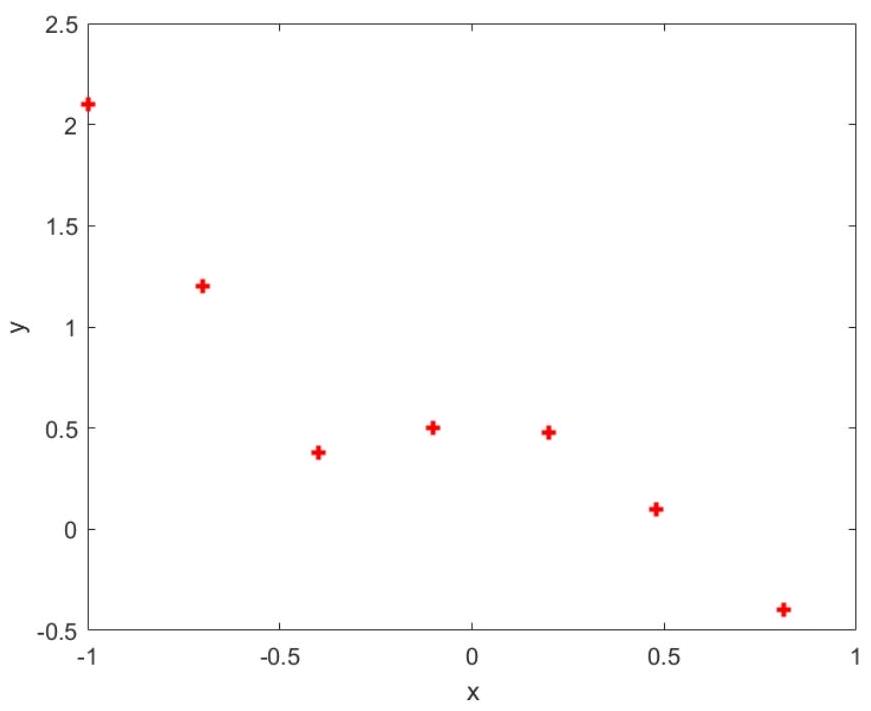
Figure 1.1 Plot of training data hw10data1.txt
hw10data1.txt is given by:
-1, 2.1
-0.7, 1.2
-0.4, 0.38
-0.1, 0.5
0.2, 0.48
0.48, 0.1
0.81, -0.4
From the plot, it seems that fitting a straight line might be too simple of an approximation. Instead, we try a fifth-order polynomial. Our hypothesis will be
\[h_{\theta}(x)=\theta^{\mathrm{T}} x=\theta_{0}+\theta_{1} x+\theta_{2} x^{2}+\theta_{3} x^{3}+\theta_{4} x^{4}+\theta_{5} x^{5} \]Since we are fitting a 5 th-order polynomial to a data set of only 7 points, overfitting is likely to occur.
To avoid this, we use regularized linear regression.
-
Write the regularized cost function;
-
Derive the gradients of the above cost function;
-
Write the gradient descent algorithm for the regularized linear regression;
-
Plot the following three figures for the regularization parameter \(\lambda=0, \lambda=1\), and \(\lambda=10\) by using the gradient descent algorithm and explain your results;
Regularized Cost Function:
The ordinary const function can be written by
\[J(\theta) = \left(y - X\theta \right)^\top \left(y - X \theta \right) \]where \(X\) is the Vandermonde matrix (\(n = 5\)), i.e.
\[\begin{bmatrix} 1 & x_1 & x_1^2 & \cdots & x_1^n \\ 1 & x_2 & x_2^2 & \cdots & x_2^n \\ \vdots & \vdots & \vdots & \ddots & \vdots \\ 1 & x_m & x_m^2 & \cdots & x_m^n \\ \end{bmatrix} \]and the regularized const fucntion is
\[J(\theta) = \frac{1}{2m} \left(y - X\theta \right)^\top \left(y - X \theta \right) +\frac{1}{2m} \lambda \theta ^\top \theta \]Gradients of the Cost Function:
To derive the gradient of (J(\theta)), we first calculate the derivative of \(J(\theta)\) without the regularization term:
\[\frac{\partial J(\theta)}{\partial \theta} = -\frac{1}{m}X^T(y - X\theta) \]And then, we calculate the derivative of the regularization term:
\[\frac{\partial}{\partial \theta} \left(\frac{\lambda}{2m} \theta^T\theta\right) = \frac{\lambda}{m} \theta \]The gradient of the regularized cost function (J(\theta)) is the sum of the gradients of the two parts:
\[\nabla J(\theta) = -\frac{1}{m}X^T(y - X\theta) + \frac{\lambda}{m} \theta \]import numpy as np
def load_x():
file_path = 'hw10data1.txt'
x = []
y = []
with open(file_path, 'r') as file:
lines = file.readlines()
for line in lines:
parts = line.strip().split(',')
x.append(float(parts[0]))
y.append(float(parts[1]))
return np.array(x), np.array(y)
x, y = load_x()
print("x array:", x)
print("y array:", y)
x array: [-1.   -0.7  -0.4  -0.1   0.2   0.48  0.81]
y array: [ 2.1   1.2   0.38  0.5   0.48  0.1  -0.4 ]
def construct_vandermonde_matrix(x, n):
    vandermonde_matrix = np.column_stack([x ** i for i in range(n)])
    return vandermonde_matrix
Gradient Descent Algorithm
def gradient_descent(X, y, theta, learning_rate, iterations, lambd):
    m = len(y)
    for _ in range(iterations):
        gradient = -1/m * X.T.dot(y - X.dot(theta)) + lambd/m * theta
        theta = theta - learning_rate * gradient
    return theta
x, y = load_x()
n = 5
X = construct_vandermonde_matrix(x, n)

# Initialize theta, learning_rate, iterations, and lambd here
theta = np.zeros(n)
learning_rate = 0.01
iterations = 1000
lambd = 0.1

# Apply the gradient descent function
theta = gradient_descent(X, y, theta, learning_rate, iterations, lambd)

print("Optimized theta values:", theta)
Optimized theta values: [ 0.35327229 -0.6234696 0.18933476 -0.61360503 0.2504074 ]
import matplotlib.pyplot as plt

def plot_fig():
    # Plotting
    x_values = np.linspace(-1, 1, 100)
    X_test = construct_vandermonde_matrix(x_values, n)
    y_values = X_test.dot(theta)

    plt.scatter(x, y, color='blue', label=f"training data")
    plt.plot(x_values, y_values, color='red', label=f"{n}th order, lambda = {lambd}")
    plt.xlabel('x')
    plt.ylabel('y')
    plt.legend()
    plt.show()
lambd = 0
theta = gradient_descent(X, y, theta, learning_rate, iterations, lambd)
plot_fig()

lambd = 1
theta = gradient_descent(X, y, theta, learning_rate, iterations, lambd)
plot_fig()

lambd = 10
theta = gradient_descent(X, y, theta, learning_rate, iterations, lambd)
plot_fig()

Logistic Regression with Gradient Descent Method
Suppose you are the product manager of the factory and you have the test results for some microchips on two different tests. From these two tests, you would like to determine whether the microchips should be accepted or rejected. To help you make the decision, you have a dataset hw10data2.txt of test results on past microchips, from which you can build a logistic regression model.
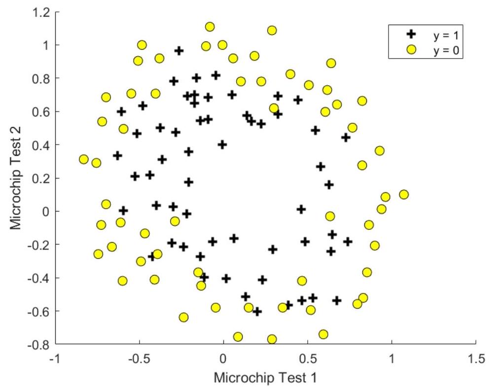
Figure 2.1 Plot of training data hw10data2. txt
Figure 2.1 shows that the dataset cannot be separated into positive and negative examples by a straight line through the plot. Therefore, a straight-forward application of logistic regression will not perform well on this dataset since logistic regression will only be able to find a linear decision boundary. One way to fit the data better is to create more features from each data point. We will map the features into all polynomial terms of \(x_{1}\) and \(x_{2}\) up to the sixth power. That means we will use the following hypothesis for the logistic regression classifier:
\[\begin{aligned} & h_{\theta}(x)=g\left(\theta^{\mathrm{T}} x\right), g(z)=\frac{1}{1+\mathrm{e}^{-z}}, \\ & \theta^{\mathrm{T}} x=\theta_{0}+\theta_{1} x_{1}+\theta_{2} x_{2}+\theta_{3} x_{1}^{2}+\theta_{4} x_{1} x_{2}+\theta_{5} x_{2}^{2} \\ & +\theta_{6} x_{1}^{3}+\theta_{7} x_{1}^{2} x_{2}+\theta_{8} x_{1} x_{2}^{2}+\theta_{9} x_{2}^{3} \\ & +\theta_{10} x_{1}^{4}+\theta_{11} x_{1}^{3} x_{2}+\theta_{12} x_{1}^{2} x_{2}^{2}+\theta_{13} x_{1} x_{2}^{3}+\theta_{14} x_{2}^{4} \\ & +\theta_{15} x_{1}^{5}+\theta_{16} x_{1}^{4} x_{2}+\theta_{17} x_{1}^{3} x_{2}^{2}+\theta_{18} x_{1}^{2} x_{2}^{3}+\theta_{19} x_{1} x_{2}^{4}+\theta_{20} x_{2}^{5} \\ & +\theta_{21} x_{1}^{6}+\theta_{22} x_{1}^{5} x_{2}+\theta_{23} x_{1}^{4} x_{2}^{2}+\theta_{24} x_{1}^{3} x_{2}^{3}+\theta_{25} x_{1}^{2} x_{2}^{4}+\theta_{26} x_{1} x_{2}^{5}+\theta_{27} x_{2}^{6} \end{aligned} \]We know that too many features may result in overfitting, so we implement regularized logistic regression to fit the data.
Regularized cost function in logistic regression
Write the regularized cost function in logistic regression;
Observe that function \(g\) is actually the sigmoid function,
The cost function is give by:
\[\begin{aligned} & \min _\theta J(\theta), \\ & J(\theta)=-\frac{1}{m} \sum_{i=1}^m\left[y^{(i)} \log h_\theta\left(x^{(i)}\right)+\left(1-y^{(i)}\right) \log \left(1-h_\theta\left(x^{(i)}\right)\right)\right]+\frac{\lambda}{2 m} \sum_{j=1}^n \theta_j^2\end{aligned} \]Gradients of the above cost function
Observe that the function \(h_\theta(x^{(i)}) = \frac{1}{1 + e^{-\theta^T x^{(i)}}}\) is the logistic (sigmoid) function.
we have some tricks for the sigmoid function, which are (function parameters are omitted)
\[\sigma' = \sigma \cdot (1 - \sigma) \]\[(\log \sigma)' = \frac{1}{e^x+1} \]\[\sigma(x) = 1-\sigma(-x) \]by applying the tricks above we ahve that
\[\begin{aligned} &\frac{\partial }{\partial x}\left((1-y^{(i)}) \log (1-\sigma(x))+y ^{(i)})\log (\sigma(x))\right) \\ = \ & y^{(i)} - \sigma(x) \end{aligned} \]So the gradient of \(J(\theta)\) is given by:
\[\frac{\partial J(\theta)}{\partial \theta_0} = \frac{1}{m} \sum_{i=1}^m \left(h_\theta(x^{(i)}) - y^{(i)}\right) x_0^{(i)} \]\[\frac{\partial J(\theta)}{\partial \theta_j} = \frac{1}{m} \sum_{i=1}^m \left(h_\theta(x^{(i)}) - y^{(i)}\right) x_j^{(i)} + \frac{\lambda}{m} \theta_j \text{ for } j = 1, \ldots, n \]where \(x^{(i)}\) represents the feature vector of the \(i\)th training example, \(y^{(i)}\) is the corresponding label, and \(\lambda\) is the regularization parameter.
Execute the gradient descent algorithm and their corresponding plots
import numpy as np

def load_x():
    file_path = 'hw10data2.txt'
    x1 = []
    x2 = []
    y = []
    with open(file_path, 'r') as file:
        lines = file.readlines()
        for line in lines:
            parts = line.strip().split(',')
            x1.append(float(parts[0]))
            x2.append(float(parts[1]))
            y.append(float(parts[2]))

    return np.array(np.transpose([x1, x2])), np.array(y)

x, y = load_x()
def construct_vandermonde_matrix(x, order):
    data_size = x.shape[0]
    vander = np.zeros((data_size, (order + 1) * (order + 2) // 2))
    for current_ind in range(data_size):
        current_x = x[current_ind, :]
        index = 0
        for n1 in range(order + 1):
            for n2 in range(order + 1 - n1):
                vander[current_ind, index] = current_x[0] ** n1 * current_x[1] ** n2
                index += 1
    return vander

X = construct_vandermonde_matrix(x, 6)
print(X.shape)
(118, 28)
def sigmoid(z):
    return 1 / (1 + np.exp(-z))

def hypothesis_function(theta, x_row):
    return sigmoid(theta.dot(x_row))

def h_wrap(theta, X):
    res = []
    for i in range(X.shape[0]):
        res.append(hypothesis_function(theta, X[i, :]))
    return np.array(res)
def gradient_descent(X, y, theta, learning_rate, iterations, lambd): # not finished yet
    m = len(y)
    for _ in range(iterations):
        gradient = np.empty((1, 28))
        tmp = h_wrap(theta, X) - y
        gradient[0] = tmp.dot(X[:, 0]) / m

        gradient = np.zeros(28)
        # print(f"gradient = {gradient}")
        for i in range(1, 28):
            # tmp = h_wrap(theta, X) - y
            # print(f"tmp.dot(X[:, i]) / m = {tmp.dot(X[:, i]) / m}")
            # print(f"lambd * theta[i] / m = {lambd * theta[i] / m}")
            gradient[i] = tmp.dot(X[:, i]) / m + lambd * theta[i] / m
        theta = theta - learning_rate * gradient
    return theta
max_order = 6
n = (1 + max_order + 1) * (max_order + 1) // 2
print(f"width of the Vandermonde matrix: {n}")
# Initialize theta, learning_rate, iterations, and lambd here
theta = np.zeros(n)
learning_rate = 0.01
iterations = 10000
lambd = 0.1

# Apply the gradient descent function
theta = gradient_descent(X, y, theta, learning_rate, iterations, lambd)

print("Optimized theta values:", theta)
width of the Vandermonde matrix: 28
Optimized theta values: [ 0.          1.24840339  0.08434246 -0.19608066 -0.9424621  -0.69907608
 -1.10322374  0.4983416  -0.97733676 -0.24856352 -0.26537115 -0.21632738
 -0.11254653 -0.79591403 -0.37502702 -0.47569472 -0.28680801 -0.31413115
  0.11819405 -0.1093652  -0.04540563 -0.00267605 -1.18512554 -0.2280036
 -0.26935639 -0.28587253 -0.01128536 -1.01289731]
import matplotlib.pyplot as plt

def plot_fig_con(lambd):
    x1_min, x1_max = x[:, 0].min() - 1, x[:, 0].max() + 1
    x2_min, x2_max = x[:, 1].min() - 1, x[:, 1].max() + 1
    xx1, xx2 = np.meshgrid(np.arange(x1_min, x1_max, 0.1),
                           np.arange(x2_min, x2_max, 0.1))

    grid = np.c_[xx1.ravel(), xx2.ravel()]
    X_grid = construct_vandermonde_matrix(grid, 6)

    probs = h_wrap(theta, X_grid)
    probs = probs.reshape(xx1.shape)

    plt.contourf(xx1, xx2, probs, alpha=0.8)
    plt.scatter(x[:, 0], x[:, 1], c=y, edgecolors='k')
    plt.xlabel('X1')
    plt.ylabel('X2')
    plt.title(f"lambda = {lambd}")
    plt.show()
import matplotlib.pyplot as plt

def plot_fig(lambd):
    plt.scatter(x[y == 0, 0], x[y == 0, 1], c='red', edgecolors='k', label='class 0: y = 0')
    plt.scatter(x[y == 1, 0], x[y == 1, 1], c='blue', edgecolors='k', label='class 1: y = 1')


    x1_min, x1_max = x[:, 0].min() - 1, x[:, 0].max() + 1
    x2_min, x2_max = x[:, 1].min() - 1, x[:, 1].max() + 1
    xx1, xx2 = np.meshgrid(np.arange(x1_min, x1_max, 0.1),
                           np.arange(x2_min, x2_max, 0.1))

    grid = np.c_[xx1.ravel(), xx2.ravel()]
    X_grid = construct_vandermonde_matrix(grid, 6)

    probs = h_wrap(theta, X_grid)
    probs = probs.reshape(xx1.shape)

    plt.contour(xx1, xx2, probs, levels=[0.5], colors='r', linestyles='dashed', label='Decision Boundary')

    plt.legend()

    plt.xlabel('X1')
    plt.ylabel('X2')
    plt.title(f"lambda = {lambd}")

    plt.show()
lambd = 0
theta = gradient_descent(X, y, theta, learning_rate, iterations, lambd)
plot_fig_con(lambd)
plot_fig(lambd)

/var/folders/3j/8tl_3gps0f77ph8f010qmqtr0000gn/T/ipykernel_6658/237325556.py:19: UserWarning: The following kwargs were not used by contour: 'label'
  plt.contour(xx1, xx2, probs, levels=[0.5], colors='r', linestyles='dashed', label='Decision Boundary')

lambd = 1
theta = gradient_descent(X, y, theta, learning_rate, iterations, lambd)
plot_fig_con(lambd)
plot_fig(lambd)

/var/folders/3j/8tl_3gps0f77ph8f010qmqtr0000gn/T/ipykernel_6658/237325556.py:19: UserWarning: The following kwargs were not used by contour: 'label'
  plt.contour(xx1, xx2, probs, levels=[0.5], colors='r', linestyles='dashed', label='Decision Boundary')

lambd = 100
theta = gradient_descent(X, y, theta, learning_rate, iterations, lambd)
plot_fig_con(lambd)
plot_fig(lambd)

/var/folders/3j/8tl_3gps0f77ph8f010qmqtr0000gn/T/ipykernel_6658/237325556.py:19: UserWarning: The following kwargs were not used by contour: 'label'
  plt.contour(xx1, xx2, probs, levels=[0.5], colors='r', linestyles='dashed', label='Decision Boundary')
