随着深度学习的发展,模型变得越来越复杂,随之而来的模型参数也越来越多,对于需要训练的模型硬件要求也越来越高。模型压缩技术就是为了解决模型使用成本的问题。通过提高推理速度,降低模型参数量和运算量。现在主流的模型压缩方法包含两大类:剪枝和量化。模型的剪枝是为了减少参数量和运算量,而量化是为了压缩数据的占用量。
(1)模型的剪枝:
剪枝的思路在工程上非常常见,在学习决策树的时候就有通过剪枝的方法来防止过拟合,同样深度学习模型剪枝就是利用这种思想,来删除收益过低的一些计算成本。
基于深度神经网络的大型预训练模型往往拥有着庞大的参数量, 然后达到SOTA的效果。但是我们参考生物的神经网络, 发现却是依靠大量稀疏的连接来完成复杂的意识活动。仿照生物的稀疏神经网络, 通过将大型网络中的稠密连接变成稀疏的连接, 在训练的过程中,逐步将权重较小的参数置为0,然后把那些权重值为0的去掉,也可以达到SOTA的效果, 就是模型的剪枝方法。
Pytorch的模型剪枝方法
- 第一种: 对特定网络模块的剪枝(Pruning Model).
- 第二种: 多参数模块的剪枝(Pruning multiple parameters).
- 第三种: 全局剪枝(GLobal pruning).
- 第四种: 用户自定义剪枝(Custom pruning).
# 第一种: 对特定网络模块的剪枝(Pruning Model).

import torch
from torch import nn
import torch.nn.utils.prune as prune
import torch.nn.functional as F

device = torch.device("cuda" if torch.cuda.is_available() else "cpu")


class LeNet(nn.Module):
    def __init__(self):
        super(LeNet, self).__init__()
        # 1: 图像的输入通道(1是黑白图像), 6: 输出通道, 3x3: 卷积核的尺寸
        self.conv1 = nn.Conv2d(1, 6, 3)
        self.conv2 = nn.Conv2d(6, 16, 3)
        self.fc1 = nn.Linear(16 * 5 * 5, 120)  # 5x5 是经历卷积操作后的图片尺寸
        self.fc2 = nn.Linear(120, 84)
        self.fc3 = nn.Linear(84, 10)

    def forward(self, x):
        x = F.max_pool2d(F.relu(self.conv1(x)), (2, 2))
        x = F.max_pool2d(F.relu(self.conv2(x)), 2)
        x = x.view(-1, int(x.nelement() / x.shape[0]))
        x = F.relu(self.fc1(x))
        x = F.relu(self.fc2(x))
        x = self.fc3(x)
        return x


model = LeNet().to(device=device)

module = model.conv1
print(list(module.named_parameters()))

print(list(module.named_buffers()))

# 第一个参数: module, 代表要进行剪枝的特定模块, 之前我们已经制定了module=model.conv1,
#             说明这里要对第一个卷积层执行剪枝.
# 第二个参数: name, 指定要对选中的模块中的哪些参数执行剪枝.
#             这里设定为name="weight", 意味着对连接网络中的weight剪枝, 而不对bias剪枝.
# 第三个参数: amount, 指定要对模型中多大比例的参数执行剪枝.
#             amount是一个介于0.0-1.0的float数值, 或者一个正整数指定剪裁掉多少条连接边.

prune.random_unstructured(module, name="weight", amount=0.3)

print(list(module.named_parameters()))
print(list(module.named_buffers()))

# 模型经历剪枝操作后, 原始的权重矩阵weight参数不见了,
# 变成了weight_orig. 并且刚刚打印为空列表的module.named_buffers(),
# 此时拥有了一个weight_mask参数.

print(module.weight)
# 经过剪枝操作后的模型, 原始的参数存放在了weight_orig中,
# 对应的剪枝矩阵存放在weight_mask中, 而将weight_mask视作掩码张量,
# 再和weight_orig相乘的结果就存放在了weight中.

# 我们可以对模型的任意子结构进行剪枝操作,
# 除了在weight上面剪枝, 还可以对bias进行剪枝.

# 第一个参数: module, 代表剪枝的对象, 此处代表LeNet中的conv1
# 第二个参数: name, 代表剪枝对象中的具体参数, 此处代表偏置量
# 第三个参数: amount, 代表剪枝的数量, 可以设置为0.0-1.0之间表示比例, 也可以用正整数表示剪枝的参数绝对数量
prune.l1_unstructured(module, name="bias", amount=3)

# 再次打印模型参数
print(list(module.named_parameters()))
print('*'*50)
print(list(module.named_buffers()))
print('*'*50)
print(module.bias)
print('*'*50)
print(module._forward_pre_hooks)

# 序列化一个剪枝模型(Serializing a pruned model):
# 对于一个模型来说, 不管是它原始的参数, 拥有的属性值, 还是剪枝的mask buffers参数
# 全部都存储在模型的状态字典中, 即state_dict()中.
# 将模型初始的状态字典打印出来
print(model.state_dict().keys())
print('*'*50)

# 对模型进行剪枝操作, 分别在weight和bias上剪枝
module = model.conv1
prune.random_unstructured(module, name="weight", amount=0.3)
prune.l1_unstructured(module, name="bias", amount=3)

# 再将剪枝后的模型的状态字典打印出来
print(model.state_dict().keys())

# 对模型执行剪枝remove操作.
# 通过module中的参数weight_orig和weight_mask进行剪枝, 本质上属于置零遮掩, 让权重连接失效.
# 具体怎么计算取决于_forward_pre_hooks函数.
# 这个remove是无法undo的, 也就是说一旦执行就是对模型参数的永久改变.

# 打印剪枝后的模型参数
print(list(module.named_parameters()))
print('*'*50)

# 打印剪枝后的模型mask buffers参数
print(list(module.named_buffers()))
print('*'*50)

# 打印剪枝后的模型weight属性值
print(module.weight)
print('*'*50)

# 打印模型的_forward_pre_hooks
print(module._forward_pre_hooks)
print('*'*50)

# 执行剪枝永久化操作remove
prune.remove(module, 'weight')
print('*'*50)

# remove后再次打印模型参数
print(list(module.named_parameters()))
print('*'*50)

# remove后再次打印模型mask buffers参数
print(list(module.named_buffers()))
print('*'*50)

# remove后再次打印模型的_forward_pre_hooks
print(module._forward_pre_hooks)

# 对模型的weight执行remove操作后, 模型参数集合中只剩下bias_orig了,
# weight_orig消失, 变成了weight, 说明针对weight的剪枝已经永久化生效.
# 对于named_buffers张量打印可以看出, 只剩下bias_mask了,
# 因为针对weight做掩码的weight_mask已经生效完毕, 不再需要保留了.
# 同理, 在_forward_pre_hooks中也只剩下针对bias做剪枝的函数了.
# 第二种: 多参数模块的剪枝(Pruning multiple parameters).
model = LeNet().to(device=device)

# 打印初始模型的所有状态字典
print(model.state_dict().keys())
print('*'*50)

# 打印初始模型的mask buffers张量字典名称
print(dict(model.named_buffers()).keys())
print('*'*50)

# 对于模型进行分模块参数的剪枝
for name, module in model.named_modules():
    # 对模型中所有的卷积层执行l1_unstructured剪枝操作, 选取20%的参数剪枝
    if isinstance(module, torch.nn.Conv2d):
        prune.l1_unstructured(module, name="weight", amount=0.2)
    # 对模型中所有全连接层执行ln_structured剪枝操作, 选取40%的参数剪枝
    elif isinstance(module, torch.nn.Linear):
        prune.ln_structured(module, name="weight", amount=0.4, n=2, dim=0)

# 打印多参数模块剪枝后的mask buffers张量字典名称
print(dict(model.named_buffers()).keys())
print('*'*50)

# 打印多参数模块剪枝后模型的所有状态字典名称
print(model.state_dict().keys())

# 对比初始化模型的状态字典和剪枝后的状态字典,
# 可以看到所有的weight参数都没有了,
# 变成了weight_orig和weight_mask的组合.
# 初始化的模型named_buffers是空列表,
# 剪枝后拥有了所有参与剪枝的参数层的weight_mask张量.
# 第三种: 全局剪枝(GLobal pruning).

# 第一种, 第二种剪枝策略本质上属于局部剪枝(local pruning)
# 更普遍也更通用的剪枝策略是采用全局剪枝(global pruning),
# 比如在整体网络的视角下剪枝掉20%的权重参数,
# 而不是在每一层上都剪枝掉20%的权重参数.
# 采用全局剪枝后, 不同的层被剪掉的百分比不同.

model = LeNet().to(device=device)

# 首先打印初始化模型的状态字典
print(model.state_dict().keys())
print('*'*50)

# 构建参数集合, 决定哪些层, 哪些参数集合参与剪枝
parameters_to_prune = (
            (model.conv1, 'weight'),
            (model.conv2, 'weight'),
            (model.fc1, 'weight'),
            (model.fc2, 'weight'),
            (model.fc3, 'weight'))

# 调用prune中的全局剪枝函数global_unstructured执行剪枝操作, 此处针对整体模型中的20%参数量进行剪枝
prune.global_unstructured(parameters_to_prune, pruning_method=prune.L1Unstructured, amount=0.2)

# 最后打印剪枝后的模型的状态字典
print(model.state_dict().keys())

model = LeNet().to(device=device)

parameters_to_prune = (
            (model.conv1, 'weight'),
            (model.conv2, 'weight'),
            (model.fc1, 'weight'),
            (model.fc2, 'weight'),
            (model.fc3, 'weight'))

prune.global_unstructured(parameters_to_prune, pruning_method=prune.L1Unstructured, amount=0.2)

print(
    "Sparsity in conv1.weight: {:.2f}%".format(
    100. * float(torch.sum(model.conv1.weight == 0))
    / float(model.conv1.weight.nelement())
    ))

print(
    "Sparsity in conv2.weight: {:.2f}%".format(
    100. * float(torch.sum(model.conv2.weight == 0))
    / float(model.conv2.weight.nelement())
    ))

print(
    "Sparsity in fc1.weight: {:.2f}%".format(
    100. * float(torch.sum(model.fc1.weight == 0))
    / float(model.fc1.weight.nelement())
    ))

print(
    "Sparsity in fc2.weight: {:.2f}%".format(
    100. * float(torch.sum(model.fc2.weight == 0))
    / float(model.fc2.weight.nelement())
    ))

print(
    "Sparsity in fc3.weight: {:.2f}%".format(
    100. * float(torch.sum(model.fc3.weight == 0))
    / float(model.fc3.weight.nelement())
    ))

print(
    "Global sparsity: {:.2f}%".format(
    100. * float(torch.sum(model.conv1.weight == 0)
               + torch.sum(model.conv2.weight == 0)
               + torch.sum(model.fc1.weight == 0)
               + torch.sum(model.fc2.weight == 0)
               + torch.sum(model.fc3.weight == 0))
         / float(model.conv1.weight.nelement()
               + model.conv2.weight.nelement()
               + model.fc1.weight.nelement()
               + model.fc2.weight.nelement()
               + model.fc3.weight.nelement())
    ))

# 当采用全局剪枝策略的时候(假定20%比例参数参与剪枝),
# 仅保证模型总体参数量的20%被剪枝掉,
# 具体到每一层的情况则由模型的具体参数分布情况来定.
# 第四种: 用户自定义剪枝(Custom pruning).
# 剪枝模型通过继承class BasePruningMethod()来执行剪枝,
# 内部有若干方法: call, apply_mask, apply, prune, remove等等.
# 一般来说, 用户只需要实现__init__, 和compute_mask两个函数即可完成自定义的剪枝规则设定.
import time
# 自定义剪枝方法的类, 一定要继承prune.BasePruningMethod
class myself_pruning_method(prune.BasePruningMethod):
    PRUNING_TYPE = "unstructured"

    # 内部实现compute_mask函数, 完成程序员自己定义的剪枝规则, 本质上就是如何去mask掉权重参数
    def compute_mask(self, t, default_mask):
        mask = default_mask.clone()
        # 此处定义的规则是每隔一个参数就遮掩掉一个, 最终参与剪枝的参数量的50%被mask掉
        mask.view(-1)[::2] = 0
        return mask

# 自定义剪枝方法的函数, 内部直接调用剪枝类的方法apply
def myself_unstructured_pruning(module, name):
    myself_pruning_method.apply(module, name)
    return module


# 实例化模型类
model = LeNet().to(device=device)

start = time.time()
# 调用自定义剪枝方法的函数, 对model中的第三个全连接层fc3中的偏置bias执行自定义剪枝
myself_unstructured_pruning(model.fc3, name="bias")

# 剪枝成功的最大标志, 就是拥有了bias_mask参数
print(model.fc3.bias_mask)

# 打印一下自定义剪枝的耗时
duration = time.time() - start
print(duration * 1000, 'ms')

# 打印出来的bias_mask张量, 完全是按照预定义的方式每隔一位遮掩掉一位,
#  0和1交替出现, 后续执行remove操作的时候,
# 原始的bias_orig中的权重就会同样的被每隔一位剪枝掉一位.
(2)模型的量化:
量化就是将这些连续的权值进一步稀疏化、离散化。进行离散化之后,相较于原来的连续稠密的值就可以用离散的值来表示了。例如,现在有256个值,是从0到255的整数,那么可以看出这一组数字从统计上来看熵是非常大的,因为分布非常均匀。你是很难对这样的数字表示进行压缩的,要想表示出它们当中的每一个,你必须用8bit的数据来表示。可是,如果这些数字集中在某些数字周围呢?比如256个值里面有56个是8,100个是7,100个9,情况会有什么不同吗?从直观感觉上了看,熵肯定是要小很多的,因为确定性高了很多。那么我们如果用3bit来表示它的中心位置8,再用2bit表示偏移量——1表示+1,0表示无偏移,-1表示-1。那么数据的存储空间又有很大的节省。原来的256个值,每个是8bit,那么一共需要2048个字节才能把数据全都记下来。而用了新方法后,每个值都可以表示为3bit的中心点和2bit的偏移量的大小,那么就变成了5bit来表示一个数字,一共需要1280的字节就够了。
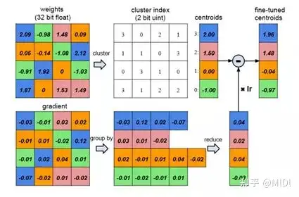
把所有的权值尝试着聚拢到一起,就是尝试找到多个簇,并找的各簇的中心点,在这个图上示意是找到了4个不同的中心点,然后用2bit的信息来表示中心点的编号。然后每个中心点的具体位置具体在列表中标出来(centroids),就是2.00,1.50,0.00和-1.00这几个值。这样记录中心点的矩阵就会小很多,这个过程就叫量化。相较于剪枝而言,量化更容易推广到不同的网络结构中。以下通过在CIFAR-10数据上进行模型的量化,最终结果如下:
config.py
import torch

init_epoch_lr = [(10, 0.01), (20, 0.001), (20, 0.0001)]
sparisity_list = [50, 60, 70, 80, 90]

finetune_epoch_lr = [
    [(3, 0.01),  (3, 0.001),  (3, 0.0001)],
    [(6, 0.01),  (6, 0.001),  (6, 0.0001)],
    [(9, 0.01),  (9, 0.001),  (9, 0.0001)],
    [(12, 0.01), (12, 0.001), (12, 0.0001)],
    [(20, 0.01), (20, 0.001), (20, 0.0001)]
]

checkpoint = 'checkpoint'

batch_size = 128
device = torch.device('cuda:0' if torch.cuda.is_available() else 'cpu')
model.py
from torch import nn


class VGG_prunable(nn.Module):
    def __init__(self, cfg):
        super(VGG_prunable, self).__init__()
        self.features = self._make_layers(cfg)
        self.classifier = nn.Linear(cfg[-2], 10)

    def _make_layers(self, cfg):
        layers = []
        in_channels = 3
        for x in cfg:
            if x == 'M':
                layers += [nn.MaxPool2d(kernel_size=2, stride=2)]
            else:
                layers += [
                    nn.Conv2d(in_channels=in_channels,
                              out_channels=x, kernel_size=3, padding=1),
                    nn.BatchNorm2d(x),
                    nn.ReLU(inplace=True)
                ]
                in_channels = x
        layers += [nn.AvgPool2d(kernel_size=1, stride=1)]
        return nn.Sequential(*layers)

    def forward(self, x):
        out = self.features(x)
        out = out.view(out.size(0), -1)
        out = self.classifier(out)
        return out


def VGG_11_prune(cfg=None):
    if cfg is None:
        cfg = [64, 'M', 128, 'M', 256, 256, 'M', 512, 512, 'M', 512, 512, 'M']
    return VGG_prunable(cfg)


if __name__ == '__main__':
    print(VGG_11_prune())

##################################################################################
VGG_prunable(
  (features): Sequential(
    (0): Conv2d(3, 64, kernel_size=(3, 3), stride=(1, 1), padding=(1, 1))
    (1): BatchNorm2d(64, eps=1e-05, momentum=0.1, affine=True, track_running_stats=True)
    (2): ReLU(inplace=True)
    (3): MaxPool2d(kernel_size=2, stride=2, padding=0, dilation=1, ceil_mode=False)
    (4): Conv2d(64, 128, kernel_size=(3, 3), stride=(1, 1), padding=(1, 1))
    (5): BatchNorm2d(128, eps=1e-05, momentum=0.1, affine=True, track_running_stats=True)
    (6): ReLU(inplace=True)
    (7): MaxPool2d(kernel_size=2, stride=2, padding=0, dilation=1, ceil_mode=False)
    (8): Conv2d(128, 256, kernel_size=(3, 3), stride=(1, 1), padding=(1, 1))
    (9): BatchNorm2d(256, eps=1e-05, momentum=0.1, affine=True, track_running_stats=True)
    (10): ReLU(inplace=True)
    (11): Conv2d(256, 256, kernel_size=(3, 3), stride=(1, 1), padding=(1, 1))
    (12): BatchNorm2d(256, eps=1e-05, momentum=0.1, affine=True, track_running_stats=True)
    (13): ReLU(inplace=True)
    (14): MaxPool2d(kernel_size=2, stride=2, padding=0, dilation=1, ceil_mode=False)
    (15): Conv2d(256, 512, kernel_size=(3, 3), stride=(1, 1), padding=(1, 1))
    (16): BatchNorm2d(512, eps=1e-05, momentum=0.1, affine=True, track_running_stats=True)
    (17): ReLU(inplace=True)
    (18): Conv2d(512, 512, kernel_size=(3, 3), stride=(1, 1), padding=(1, 1))
    (19): BatchNorm2d(512, eps=1e-05, momentum=0.1, affine=True, track_running_stats=True)
    (20): ReLU(inplace=True)
    (21): MaxPool2d(kernel_size=2, stride=2, padding=0, dilation=1, ceil_mode=False)
    (22): Conv2d(512, 512, kernel_size=(3, 3), stride=(1, 1), padding=(1, 1))
    (23): BatchNorm2d(512, eps=1e-05, momentum=0.1, affine=True, track_running_stats=True)
    (24): ReLU(inplace=True)
    (25): Conv2d(512, 512, kernel_size=(3, 3), stride=(1, 1), padding=(1, 1))
    (26): BatchNorm2d(512, eps=1e-05, momentum=0.1, affine=True, track_running_stats=True)
    (27): ReLU(inplace=True)
    (28): MaxPool2d(kernel_size=2, stride=2, padding=0, dilation=1, ceil_mode=False)
    (29): AvgPool2d(kernel_size=1, stride=1, padding=0)
  )
  (classifier): Linear(in_features=512, out_features=10, bias=True)
)
##################################################################################
base_train.py
from config import device, checkpoint, init_epoch_lr
from data import trainloader, trainset, testloader, testset
from model import VGG_11_prune
import torch
from torch import optim
from torch.utils.tensorboard import SummaryWriter
import os
from tqdm import tqdm


def train_epoch(net, optimizer, crition):
    epoch_loss = 0.0
    epoch_acc = 0.0
    for j, (img, label) in tqdm(enumerate(trainloader)):
        img, label = img.to(device), label.to(device)
        out = net(img)
        optimizer.zero_grad()
        loss = crition(out, label)
        loss.backward()
        optimizer.step()
        pred = torch.argmax(out, dim=1)
        acc = torch.sum(pred == label)
        epoch_loss += loss.item()
        epoch_acc += acc.item()

    epoch_acc /= len(trainset)
    epoch_loss /= len(trainloader)
    print('epoch loss :{:8f} epoch acc :{:8f}'.format(epoch_loss, epoch_acc))
    return epoch_acc, epoch_loss, net


def validation(net, criteron):
    with torch.no_grad():
        test_loss = 0.0
        test_acc = 0.0
        for k, (img, label) in tqdm(enumerate(testloader)):
            img, label = img.to(device), label.to(device)
            out = net(img)
            loss = criteron(out, label)
            pred = torch.argmax(out, dim=1)
            acc = torch.sum(pred == label)
            test_loss += loss.item()
            test_acc += acc.item()
        test_acc /= len(testset)
        test_loss /= len(testloader)
        print('test loss :{:8f} test acc :{:8f}'.format(test_loss, test_acc))
        return test_acc, test_loss


def init_train(net):
    if os.path.exists(os.path.join(checkpoint, 'best_model.pth')):
        save_model = torch.load(os.path.join(checkpoint, 'best_model.pth'))
        net.load_state_dict(save_model['net'])
        if save_model['best_accuracy'] > 0.9:
            print('break init train')
            return
        best_accuracy = save_model['best_accuracy']
        best_loss = save_model['best_loss']
    else:
        best_accuracy = 0.0
        best_loss = 10.0
    writer = SummaryWriter('logs/')
    criteron = torch.nn.CrossEntropyLoss()

    for i, (num_epoch, lr) in enumerate(init_epoch_lr):
        optimizer = optim.SGD(net.parameters(), lr=lr, weight_decay=0.0001, momentum=0.9)
        for epoch in range(num_epoch):
            print('epoch: {}'.format(epoch))
            epoch_acc, epoch_loss, net = train_epoch(net, optimizer, criteron)
            writer.add_scalar('epoch_acc', epoch_acc,
                              sum([e[0] for e in init_epoch_lr[:i]])+epoch)
            writer.add_scalar('epoch_loss', epoch_loss,
                              sum([e[0] for e in init_epoch_lr[:i]]) + epoch)

            test_acc, test_loss = validation(net, criteron)
            if test_loss <= best_loss:
                if test_acc >= best_accuracy:
                    best_accuracy = test_acc

                best_loss = test_loss
                best_model_weights = net.state_dict().copy()
                best_model_params = optimizer.state_dict().copy()
                torch.save(
                    {
                        'net': best_model_weights,
                        'optimizer': best_model_params,
                        'best_accuracy': best_accuracy,
                        'best_loss': best_loss
                    },
                    os.path.join(checkpoint, 'best_model.pth')
                )

            writer.add_scalar('test_acc', test_acc,
                              sum([e[0] for e in init_epoch_lr[:i]]) + epoch)
            writer.add_scalar('test_loss', test_loss,
                              sum([e[0] for e in init_epoch_lr[:i]]) + epoch)

    writer.close()
    return net


if __name__ == '__main__':
    net = VGG_11_prune().to(device)
    init_train(net)
训练完成之后,会在checkpoint文件下生成模型

之后对训练好的模型参数进行量化,代码如下:
quantize.py
import torch
import os
from copy import deepcopy
from collections import OrderedDict
import matplotlib.pyplot as plt
from model import VGG_11_prune
from base_train import validation
from config import checkpoint, device
# 量化权重
def signed_quantize(x, bits, bias=None):
min_val, max_val = x.min(), x.max()
n = 2.0 ** (bits -1)
scale = max(abs(min_val), abs(max_val)) / n
qx = torch.floor(x / scale)
if bias is not None:
qb = torch.floor(bias / scale)
return qx, qb
else:
return qx
# 对模型整体进行量化
def scale_quant_model(model, bits):
net = deepcopy(model)
params_quant = OrderedDict()
params_save = OrderedDict()
for k, v in model.state_dict().items():
if 'classifier' not in k and 'num_batches' not in k and 'running' not in k:
if 'weight' in k:
weight = v
bias_name = k.replace('weight', 'bias')
try:
bias = model.state_dict()[bias_name]
w, b = signed_quantize(weight, bits, bias)
params_quant[k] = w
params_quant[bias_name] = b
if bits > 8 and bits <= 16:
params_save[k] = w.short()
params_save[bias_name] = b.short()
elif bits >1 and bits <= 8:
params_save[k] = w.char()
params_save[bias_name] = b.char()
elif bits == 1:
params_save[k] = w.bool()
params_save[bias_name] = b.bool()
except:
w = signed_quantize(w, bits)
params_quant[k] = w
params_save[k] = w.char()
else:
params_quant[k] = v
params_save[k] = v
net.load_state_dict(params_quant)
return net, params_save
if __name__ == '__main__':
pruned = False
if pruned:
channels = [17, 'M', 77, 'M', 165, 182, 'M', 338, 337, 'M', 360, 373, 'M']
net = VGG_11_prune(channels).to(device)
net.load_state_dict(
torch.load(
os.path.join(checkpoint, 'best_retrain_model.pth'))['compressed_net'])
else:
net = VGG_11_prune().to(device)
net.load_state_dict(
torch.load(
os.path.join(checkpoint, 'best_model.pth'), map_location=torch.device('cpu')
)['net']
)
validation(net, torch.nn.CrossEntropyLoss())
accuracy_list = []
bit_list = [16, 12, 8, 6, 4, 3, 2, 1]
for bit in bit_list:
print('{} bit'.format(bit))
scale_quantized_model, params = scale_quant_model(net, bit)
print('validation: ', end='\t')
accuracy, _ = validation(scale_quantized_model, torch.nn.CrossEntropyLoss())
accuracy_list.append(accuracy)
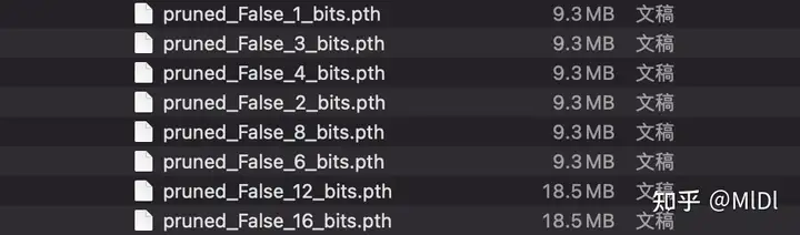
torch.save(params,
os.path.join(checkpoint, 'pruned_{}_{}_bits.pth'.format(pruned, bit)))
plt.plot(bit_list, accuracy_list)
plt.savefig('img/quantize_pruned:{}.jpg'.format(pruned))
plt.show()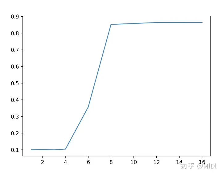
test loss :0.426187 test acc :0.862100
16 bit
validation: 	[W ParallelNative.cpp:212] Warning: Cannot set number of intraop threads after parallel work has started or after set_num_threads call when using native parallel backend (function set_num_threads)
0it [00:00, ?it/s][W ParallelNative.cpp:212] Warning: Cannot set number of intraop threads after parallel work has started or after set_num_threads call when using native parallel backend (function set_num_threads)
79it [01:14,  1.06it/s]
test loss :10474.145823 test acc :0.863400
12 bit
validation: 	[W ParallelNative.cpp:212] Warning: Cannot set number of intraop threads after parallel work has started or after set_num_threads call when using native parallel backend (function set_num_threads)
0it [00:00, ?it/s][W ParallelNative.cpp:212] Warning: Cannot set number of intraop threads after parallel work has started or after set_num_threads call when using native parallel backend (function set_num_threads)
79it [01:15,  1.04it/s]
test loss :659.361133 test acc :0.863300
8 bit
validation: 	[W ParallelNative.cpp:212] Warning: Cannot set number of intraop threads after parallel work has started or after set_num_threads call when using native parallel backend (function set_num_threads)
0it [00:00, ?it/s][W ParallelNative.cpp:212] Warning: Cannot set number of intraop threads after parallel work has started or after set_num_threads call when using native parallel backend (function set_num_threads)
79it [01:14,  1.06it/s]
test loss :48.506328 test acc :0.851800
6 bit
validation: 	[W ParallelNative.cpp:212] Warning: Cannot set number of intraop threads after parallel work has started or after set_num_threads call when using native parallel backend (function set_num_threads)
0it [00:00, ?it/s][W ParallelNative.cpp:212] Warning: Cannot set number of intraop threads after parallel work has started or after set_num_threads call when using native parallel backend (function set_num_threads)
79it [01:14,  1.07it/s]
test loss :44.048244 test acc :0.356100
4 bit
validation: 	[W ParallelNative.cpp:212] Warning: Cannot set number of intraop threads after parallel work has started or after set_num_threads call when using native parallel backend (function set_num_threads)
0it [00:00, ?it/s][W ParallelNative.cpp:212] Warning: Cannot set number of intraop threads after parallel work has started or after set_num_threads call when using native parallel backend (function set_num_threads)
79it [01:15,  1.05it/s]
test loss :5.035617 test acc :0.103500
3 bit
validation: 	[W ParallelNative.cpp:212] Warning: Cannot set number of intraop threads after parallel work has started or after set_num_threads call when using native parallel backend (function set_num_threads)
0it [00:00, ?it/s][W ParallelNative.cpp:212] Warning: Cannot set number of intraop threads after parallel work has started or after set_num_threads call when using native parallel backend (function set_num_threads)
79it [01:14,  1.06it/s]
test loss :2.572487 test acc :0.099700
2 bit
validation: 	[W ParallelNative.cpp:212] Warning: Cannot set number of intraop threads after parallel work has started or after set_num_threads call when using native parallel backend (function set_num_threads)
0it [00:00, ?it/s][W ParallelNative.cpp:212] Warning: Cannot set number of intraop threads after parallel work has started or after set_num_threads call when using native parallel backend (function set_num_threads)
79it [01:14,  1.06it/s]
test loss :2.301575 test acc :0.101000
1 bit
validation: 	[W ParallelNative.cpp:212] Warning: Cannot set number of intraop threads after parallel work has started or after set_num_threads call when using native parallel backend (function set_num_threads)
0it [00:00, ?it/s][W ParallelNative.cpp:212] Warning: Cannot set number of intraop threads after parallel work has started or after set_num_threads call when using native parallel backend (function set_num_threads)
79it [01:13,  1.07it/s]
test loss :2.303252 test acc :0.100000
由上图可以看到,将参数量化到int8,模型的精度基本没有发生较大的变化,同时模型的大小也缩小为了原来的1/8,基本很好的完成了模型的压缩效果。
标签:剪枝,set,weight,压缩,threads,print,量化,model From: https://www.cnblogs.com/kn-zheng/p/18051960