#1.数据建模
import pandas as pd
import numpy as np
import matplotlib.pyplot as plt # python绘图库可以与numpy一起使用
import seaborn as sns #基于python的图形可视化库,更加方便快捷
from IPython.display import Image
data = pd.read_csv('clear_data.csv')#清洗后的数据
train = pd.read_csv('train.csv')
data.shape,train.shape#查看清洗先后的数据差别
((891, 11), (891, 12))
data.head(2)
| PassengerId | Pclass | Age | SibSp | Parch | Fare | Sex_female | Sex_male | Embarked_C | Embarked_Q | Embarked_S | |
|---|---|---|---|---|---|---|---|---|---|---|---|
| 0 | 0 | 3 | 22.0 | 1 | 0 | 7.2500 | 0 | 1 | 0 | 0 | 1 |
| 1 | 1 | 1 | 38.0 | 1 | 0 | 71.2833 | 1 | 0 | 1 | 0 | 0 |
train.head(2)
| PassengerId | Survived | Pclass | Name | Sex | Age | SibSp | Parch | Ticket | Fare | Cabin | Embarked | |
|---|---|---|---|---|---|---|---|---|---|---|---|---|
| 0 | 1 | 0 | 3 | Braund, Mr. Owen Harris | male | 22.0 | 1 | 0 | A/5 21171 | 7.2500 | NaN | S |
| 1 | 2 | 1 | 1 | Cumings, Mrs. John Bradley (Florence Briggs Th... | female | 38.0 | 1 | 0 | PC 17599 | 71.2833 | C85 | C |
#监督学习:从标记的数据来进行机器学习的任务
#无监督学习:是从未进行标记和分类的数据进行机器学习的任务
Image('sklearn.png')#调出sklearn模型算法选择路径

# 数据拟合又称曲线拟合,俗称拉曲线,是一种把现有数据透过数学方法来代入一条数式的表示方式。
# 科学和工程问题可以通过诸如采样、实验等方法获得若干离散的数据,
# 根据这些数据,我们往往希望得到一个连续的函数(也就是曲线)或者更加密集的离散方程与已知数据相吻合,这过程就叫做拟合(fitting)

# 欠拟合,正确拟合,过拟合
#切割训练集和测试集,防止出现过拟合情况
# 数据集划分的三种方法:流出法,交叉验证法,自助法
#将数据集使用流出法划分为,自变量和因变量
X=data
y=train['Survived']
#按比例切割训练集和测试集(一般测试集为30%,25%,20%,15%,10%)
#sklearn中的切割数据集方法为train_test_split
from sklearn.model_selection import train_test_split
train_test_split?
#通过该命令来查看函数文档
[1;31mSignature:[0m
[0mtrain_test_split[0m[1;33m([0m[1;33m
[0m [1;33m*[0m[0marrays[0m[1;33m,[0m[1;33m
[0m [0mtest_size[0m[1;33m=[0m[1;32mNone[0m[1;33m,[0m[1;33m
[0m [0mtrain_size[0m[1;33m=[0m[1;32mNone[0m[1;33m,[0m[1;33m
[0m [0mrandom_state[0m[1;33m=[0m[1;32mNone[0m[1;33m,[0m[1;33m
[0m [0mshuffle[0m[1;33m=[0m[1;32mTrue[0m[1;33m,[0m[1;33m
[0m [0mstratify[0m[1;33m=[0m[1;32mNone[0m[1;33m,[0m[1;33m
[0m[1;33m)[0m[1;33m[0m[1;33m[0m[0m
[1;31mDocstring:[0m
Split arrays or matrices into random train and test subsets.
Quick utility that wraps input validation and
``next(ShuffleSplit().split(X, y))`` and application to input data
into a single call for splitting (and optionally subsampling) data in a
oneliner.
Read more in the :ref:`User Guide <cross_validation>`.
Parameters
----------
*arrays : sequence of indexables with same length / shape[0]
Allowed inputs are lists, numpy arrays, scipy-sparse
matrices or pandas dataframes.
test_size : float or int, default=None
If float, should be between 0.0 and 1.0 and represent the proportion
of the dataset to include in the test split. If int, represents the
absolute number of test samples. If None, the value is set to the
complement of the train size. If ``train_size`` is also None, it will
be set to 0.25.
train_size : float or int, default=None
If float, should be between 0.0 and 1.0 and represent the
proportion of the dataset to include in the train split. If
int, represents the absolute number of train samples. If None,
the value is automatically set to the complement of the test size.
random_state : int, RandomState instance or None, default=None
Controls the shuffling applied to the data before applying the split.
Pass an int for reproducible output across multiple function calls.
See :term:`Glossary <random_state>`.
shuffle : bool, default=True
Whether or not to shuffle the data before splitting. If shuffle=False
then stratify must be None.
stratify : array-like, default=None
If not None, data is split in a stratified fashion, using this as
the class labels.
Read more in the :ref:`User Guide <stratification>`.
Returns
-------
splitting : list, length=2 * len(arrays)
List containing train-test split of inputs.
.. versionadded:: 0.16
If the input is sparse, the output will be a
``scipy.sparse.csr_matrix``. Else, output type is the same as the
input type.
Examples
--------
>>> import numpy as np
>>> from sklearn.model_selection import train_test_split
>>> X, y = np.arange(10).reshape((5, 2)), range(5)
>>> X
array([[0, 1],
[2, 3],
[4, 5],
[6, 7],
[8, 9]])
>>> list(y)
[0, 1, 2, 3, 4]
>>> X_train, X_test, y_train, y_test = train_test_split(
... X, y, test_size=0.33, random_state=42)
...
>>> X_train
array([[4, 5],
[0, 1],
[6, 7]])
>>> y_train
[2, 0, 3]
>>> X_test
array([[2, 3],
[8, 9]])
>>> y_test
[1, 4]
>>> train_test_split(y, shuffle=False)
[[0, 1, 2], [3, 4]]
[1;31mFile:[0m c:\users\17006\anaconda3\lib\site-packages\sklearn\model_selection\_split.py
[1;31mType:[0m function
# 从clear_data.csv和train.csv中提取train_test_split()所需的参数
X_train, X_test, y_train, y_test = train_test_split(X, y, stratify=y, test_size=0.25,random_state=42)
#stratify=y表示按照y的种类比例进行分配(分层抽样),保证所有样本中不同种类的数据比例相同
# random_state=42表示初始化伪随机数生成器的数值为42
# test_size=0.25表示测试集的比例为25%,(默认测试集的比例是25%)
X_train.shape,X_test.shape
((668, 11), (223, 11))
223/(223+668)#测试集比例近似为25%
0.250280583613917
X_train.head()#随机种子设定伪随机数的初始值,随机种子不同生成结果也不同,反之相同时结果一样
| PassengerId | Pclass | Age | SibSp | Parch | Fare | Sex_female | Sex_male | Embarked_C | Embarked_Q | Embarked_S | |
|---|---|---|---|---|---|---|---|---|---|---|---|
| 486 | 486 | 1 | 35.0 | 1 | 0 | 90.000 | 1 | 0 | 0 | 0 | 1 |
| 238 | 238 | 2 | 19.0 | 0 | 0 | 10.500 | 0 | 1 | 0 | 0 | 1 |
| 722 | 722 | 2 | 34.0 | 0 | 0 | 13.000 | 0 | 1 | 0 | 0 | 1 |
| 184 | 184 | 3 | 4.0 | 0 | 2 | 22.025 | 1 | 0 | 0 | 0 | 1 |
| 56 | 56 | 2 | 21.0 | 0 | 0 | 10.500 | 1 | 0 | 0 | 0 | 1 |
from sklearn.linear_model import LogisticRegression#导入线性回归模型
from sklearn.ensemble import RandomForestClassifier#导入随机森林决策树模型
train['Survived'].value_counts()#0和1人数相差不大没有高度失衡
Survived
0    549
1    342
Name: count, dtype: int64
lr=LogisticRegression().fit(X_train,y_train)#LogisticRegression()用来创建模型,fit(X_train,y_train)用X,y对模型进行训练
lr#返回一个逻辑回归的模型
C:\Users\17006\anaconda3\lib\site-packages\sklearn\linear_model\_logistic.py:444: ConvergenceWarning: lbfgs failed to converge (status=1):
STOP: TOTAL NO. of ITERATIONS REACHED LIMIT.

Increase the number of iterations (max_iter) or scale the data as shown in:
    https://scikit-learn.org/stable/modules/preprocessing.html
Please also refer to the documentation for alternative solver options:
    https://scikit-learn.org/stable/modules/linear_model.html#logistic-regression
  n_iter_i = _check_optimize_result(
LogisticRegression()In a Jupyter environment, please rerun this cell to show the HTML representation or trust the notebook.
On GitHub, the HTML representation is unable to render, please try loading this page with nbviewer.org.
LogisticRegression()
print('训练集得分:{:.3f}'.format(lr.score(X_train,y_train)))#查看数据模型的得分,:.2f表示保留三位小数(训练集)
print('测试集得分:{:.3f}'.format(lr.score(X_test,y_test)))#查看数据模型的得分,:.2f表示保留三位小数(测试集)
训练集得分:0.804
测试集得分:0.771
#L1正则化,L2正则化防止数据出现过拟合的情况(限制模型复杂度,约束模型的复杂度)
lr1=LogisticRegression(C=2).fit(X_train,y_train)#C=2 C的参数值越小越能约束模型复杂度
print('训练集得分:{:.3f}'.format(lr1.score(X_train,y_train)))
print('测试集得分:{:.3f}'.format(lr1.score(X_test,y_test)))
训练集得分:0.799
测试集得分:0.776


C:\Users\17006\anaconda3\lib\site-packages\sklearn\linear_model\_logistic.py:444: ConvergenceWarning: lbfgs failed to converge (status=1):
STOP: TOTAL NO. of ITERATIONS REACHED LIMIT.

Increase the number of iterations (max_iter) or scale the data as shown in:
    https://scikit-learn.org/stable/modules/preprocessing.html
Please also refer to the documentation for alternative solver options:
    https://scikit-learn.org/stable/modules/linear_model.html#logistic-regression
  n_iter_i = _check_optimize_result(
lr2=LogisticRegression(class_weight='balanced').fit(X_train,y_train)#class_weight='balanced'表示不考虑权重。
# (某种类型样本量越多,则权重越低,样本量越少,则权重越高)
print('训练集得分:{:.3f}'.format(lr2.score(X_train,y_train)))
print('测试集得分:{:.3f}'.format(lr2.score(X_test,y_test)))
训练集得分:0.787
测试集得分:0.771


C:\Users\17006\anaconda3\lib\site-packages\sklearn\linear_model\_logistic.py:444: ConvergenceWarning: lbfgs failed to converge (status=1):
STOP: TOTAL NO. of ITERATIONS REACHED LIMIT.

Increase the number of iterations (max_iter) or scale the data as shown in:
    https://scikit-learn.org/stable/modules/preprocessing.html
Please also refer to the documentation for alternative solver options:
    https://scikit-learn.org/stable/modules/linear_model.html#logistic-regression
  n_iter_i = _check_optimize_result(
# 随机森林由多个决策树组成结果由决策树的平均值来决定
rf=RandomForestClassifier().fit(X_train,y_train)#RandomForestClassifier()创建随机森林模型
print('训练集得分:{:.3f}'.format(rf.score(X_train,y_train)))
print('测试集得分:{:.3f}'.format(rf.score(X_test,y_test)))
训练集得分:1.000
测试集得分:0.803
rf1=RandomForestClassifier(n_estimators=50).fit(X_train,y_train)#n_estimators=50决策树数量默认为100
print('训练集得分:{:.3f}'.format(rf1.score(X_train,y_train)))
print('测试集得分:{:.3f}'.format(rf1.score(X_test,y_test)))
训练集得分:1.000
测试集得分:0.767
rf2=RandomForestClassifier(max_depth=5).fit(X_train,y_train)#max_depth=5决策树的最大深度默认为0
print('训练集得分:{:.3f}'.format(rf2.score(X_train,y_train)))
print('测试集得分:{:.3f}'.format(rf2.score(X_test,y_test)))
训练集得分:0.867
测试集得分:0.780
rf3=RandomForestClassifier(bootstrap=False).fit(X_train,y_train)#bootstrap=False是否放回抽样,默认为True(False表示不放回)
print('训练集得分:{:.3f}'.format(rf3.score(X_train,y_train)))
print('测试集得分:{:.3f}'.format(rf3.score(X_test,y_test)))
训练集得分:1.000
测试集得分:0.776
rf4=RandomForestClassifier(oob_score=True).fit(X_train,y_train)
#oob_score=True通过bootstrap (有放回的随机抽样) 的抽样方式进行T次抽样每次抽样产生样本数为n的采样集,进入到并行的T个决策树中
# 把这T和oob_score平均,最终得到的就是整个随机森林的oob_score(即决定系数)
# 默认为False(False表示不进行上述操作)
print('训练集得分:{:.3f}'.format(rf4.score(X_train,y_train)))
print('测试集得分:{:.3f}'.format(rf4.score(X_test,y_test)))
训练集得分:1.000
测试集得分:0.803
#线性多元分类
lr.predict(X_train)#训练集样本的预测标签(1为存活)
array([1, 0, 0, 1, 1, 0, 0, 0, 1, 0, 0, 0, 0, 0, 0, 0, 0, 1, 0, 0, 0, 0,
       0, 0, 0, 0, 1, 0, 1, 0, 1, 1, 1, 1, 0, 1, 1, 1, 0, 1, 0, 0, 1, 1,
       0, 1, 0, 1, 1, 0, 0, 0, 1, 1, 0, 0, 1, 0, 0, 0, 0, 1, 1, 0, 0, 0,
       1, 0, 0, 1, 0, 1, 1, 0, 0, 0, 0, 0, 0, 0, 0, 0, 0, 0, 0, 0, 0, 0,
       1, 0, 0, 1, 0, 0, 1, 1, 0, 1, 0, 1, 1, 0, 0, 0, 1, 0, 0, 1, 1, 0,
       0, 1, 0, 0, 1, 1, 1, 0, 0, 0, 1, 0, 0, 0, 0, 0, 0, 1, 1, 1, 1, 1,
       0, 0, 0, 1, 0, 0, 0, 0, 0, 1, 0, 1, 1, 1, 0, 0, 0, 0, 1, 1, 0, 1,
       0, 0, 1, 0, 0, 0, 0, 1, 1, 1, 0, 1, 0, 0, 1, 0, 0, 1, 0, 0, 0, 1,
       1, 0, 0, 1, 0, 0, 1, 1, 0, 1, 0, 0, 1, 0, 0, 0, 0, 1, 1, 1, 0, 0,
       0, 0, 0, 0, 1, 0, 0, 1, 1, 0, 0, 1, 0, 0, 0, 0, 1, 0, 0, 0, 1, 0,
       0, 0, 0, 0, 0, 0, 1, 0, 0, 1, 0, 0, 0, 0, 0, 0, 0, 0, 1, 0, 1, 1,
       0, 1, 1, 1, 1, 0, 0, 1, 0, 0, 0, 0, 1, 0, 1, 0, 1, 0, 0, 1, 0, 0,
       1, 0, 1, 1, 0, 1, 0, 1, 1, 1, 0, 1, 0, 0, 0, 0, 0, 1, 0, 0, 1, 1,
       0, 0, 1, 1, 0, 0, 0, 0, 1, 0, 0, 0, 0, 0, 1, 1, 0, 0, 0, 0, 1, 0,
       1, 0, 0, 0, 0, 0, 0, 0, 0, 0, 0, 0, 0, 0, 0, 0, 1, 1, 0, 1, 0, 0,
       1, 1, 0, 1, 1, 1, 0, 1, 0, 1, 0, 0, 0, 0, 0, 0, 1, 0, 0, 0, 0, 0,
       0, 0, 0, 0, 1, 0, 0, 1, 0, 1, 0, 0, 1, 1, 1, 0, 0, 0, 0, 0, 0, 0,
       0, 0, 0, 0, 0, 0, 1, 0, 0, 0, 0, 0, 0, 0, 1, 1, 1, 0, 0, 0, 0, 0,
       0, 1, 0, 1, 0, 0, 0, 0, 1, 0, 0, 0, 1, 1, 0, 0, 0, 0, 0, 1, 0, 0,
       0, 1, 1, 0, 0, 0, 1, 1, 0, 0, 1, 0, 1, 0, 1, 0, 0, 1, 0, 0, 1, 1,
       1, 1, 0, 0, 0, 0, 0, 0, 0, 0, 1, 1, 0, 0, 1, 0, 0, 0, 0, 0, 0, 1,
       0, 0, 0, 1, 1, 1, 0, 1, 0, 0, 1, 1, 1, 0, 0, 1, 1, 0, 0, 0, 0, 0,
       0, 1, 0, 0, 1, 0, 1, 0, 0, 0, 0, 0, 0, 1, 0, 1, 0, 0, 0, 1, 0, 0,
       0, 1, 0, 1, 1, 0, 1, 1, 0, 0, 0, 0, 0, 0, 0, 1, 1, 0, 1, 0, 1, 1,
       1, 1, 1, 0, 1, 0, 0, 0, 1, 0, 1, 1, 1, 0, 0, 0, 1, 0, 1, 0, 0, 0,
       0, 0, 1, 0, 1, 0, 0, 0, 1, 0, 1, 0, 1, 1, 1, 0, 0, 0, 0, 0, 0, 1,
       1, 1, 0, 0, 0, 0, 0, 0, 0, 0, 1, 0, 0, 1, 0, 1, 0, 0, 0, 1, 0, 1,
       0, 0, 0, 0, 1, 0, 0, 1, 1, 0, 1, 0, 0, 0, 0, 0, 0, 0, 1, 1, 0, 0,
       0, 0, 1, 1, 1, 0, 1, 0, 1, 0, 1, 1, 0, 0, 1, 0, 1, 0, 1, 0, 1, 1,
       0, 0, 0, 1, 1, 0, 0, 1, 0, 0, 0, 0, 1, 0, 0, 1, 0, 1, 0, 1, 0, 1,
       0, 1, 0, 0, 1, 0, 0, 0], dtype=int64)
lr.predict_proba(X_train)#训练集样本的存活和死亡概率
array([[0.08612485, 0.91387515],
       [0.79027322, 0.20972678],
       [0.80569693, 0.19430307],
       ...,
       [0.53461498, 0.46538502],
       [0.72046392, 0.27953608],
       [0.87780208, 0.12219792]])
#2.评估数据模型
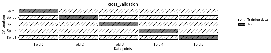
# 交叉验证(cross-validation)是一种评估泛化性能的统计学方法,它比单次划分训练集和测试集的方法更加稳定、全面。
# 在交叉验证中,数据被多次划分,并且需要训练多个模型。
# 最常用的交叉验证是 k 折交叉验证(k-fold cross-validation),其中 k 是由用户指定的数字,通常取 5 或 10
# 准确率(precision)度量的是被预测为正例的样本中有多少是真正的正例
# 召回率(recall)度量的是正类样本中有多少被预测为正类
# f-分数是准确率与召回率的调和平均
Image('Snipaste_2020-01-05_16-37-56.png')#五折交叉验证(将数据分为5等分,一份做测试数据,四分做训练数据),并进行10次运算。
from sklearn.model_selection import cross_val_score#导入交叉验证的函数
lr=LogisticRegression().fit(X_train,y_train)
score=cross_val_score(lr,X_train,y_train,cv=10)#cv=10,10折验证模型,生成结果为相应数据的准确率(10次运算)
print(score)
print(score.mean())#计算平均值
[0.80597015 0.71641791 0.80597015 0.73134328 0.91044776 0.7761194
 0.88059701 0.76119403 0.81818182 0.77272727]
0.7978968792401628


C:\Users\17006\anaconda3\lib\site-packages\sklearn\linear_model\_logistic.py:444: ConvergenceWarning: lbfgs failed to converge (status=1):
STOP: TOTAL NO. of ITERATIONS REACHED LIMIT.

Increase the number of iterations (max_iter) or scale the data as shown in:
    https://scikit-learn.org/stable/modules/preprocessing.html
Please also refer to the documentation for alternative solver options:
    https://scikit-learn.org/stable/modules/linear_model.html#logistic-regression
  n_iter_i = _check_optimize_result(
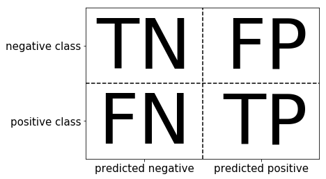
#混淆矩阵
# 混淆矩阵也称误差矩阵,是表示精度评价的一种标准格式,用n行n列的矩阵形式来表示。
Image('Snipaste_2020-01-05_16-38-26.png')
# TN:负的类预测为负的,即真的负类
# FP:假的被预测为真的,假的正类
# FN:真的被预测为假的,假的负类
# TP:真的被预测为真的,真的正类
#二元分类的混淆矩阵
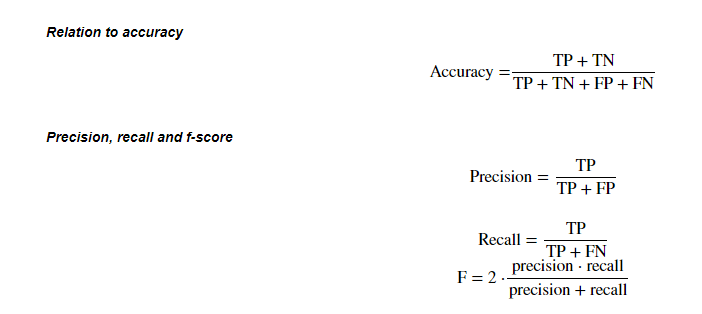
Image('Snipaste_2020-01-05_16-39-27.png')#整体准确率 (Accuracy,准确率),正类检测的正确率(Precision,精确度),召回率(Recall),f-分数计算方法
#F1分数,又称平衡F分数,是精确率与召回率的调和平均数(2/(1/P+1/R))
#使用F1平均数可以更加直观的反映一个模型的好坏,即运用加权的手段整合精确度和召回率
# FPR=FP/(FP+TN)(假正率(False Positive Rate,FPR))
# TPR=TP/(TP+FN)(真正率,True Positive Rate, TPR)
from sklearn.metrics import confusion_matrix
from sklearn.metrics import classification_report#导入混淆矩阵相关模块
lr=LogisticRegression().fit(X_train,y_train)
y_pred=lr.predict(X_train)
confusion_matrix(y_train,y_pred,labels=[0,1])#横向行表示训练集,纵向列表示预测集
#如下的意思为:y_train={'0':358+54,'1':179+77} y_pred={'0':358+77,'1':179+54}
C:\Users\17006\anaconda3\lib\site-packages\sklearn\linear_model\_logistic.py:444: ConvergenceWarning: lbfgs failed to converge (status=1):
STOP: TOTAL NO. of ITERATIONS REACHED LIMIT.

Increase the number of iterations (max_iter) or scale the data as shown in:
    https://scikit-learn.org/stable/modules/preprocessing.html
Please also refer to the documentation for alternative solver options:
    https://scikit-learn.org/stable/modules/linear_model.html#logistic-regression
  n_iter_i = _check_optimize_result(


array([[358,  54],
       [ 77, 179]], dtype=int64)
y_train.value_counts()
Survived
0    412
1    256
Name: count, dtype: int64
target_name=['死亡人数','生存人数']
print(classification_report(y_train,y_pred,target_names=target_name,labels=[0,1]))#target_names=target_name将[0,1]替换成['死亡人数','生存人数']
              precision    recall  f1-score   support

        死亡人数       0.82      0.87      0.85       412
        生存人数       0.77      0.70      0.73       256

    accuracy                           0.80       668
   macro avg       0.80      0.78      0.79       668
weighted avg       0.80      0.80      0.80       668
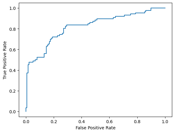
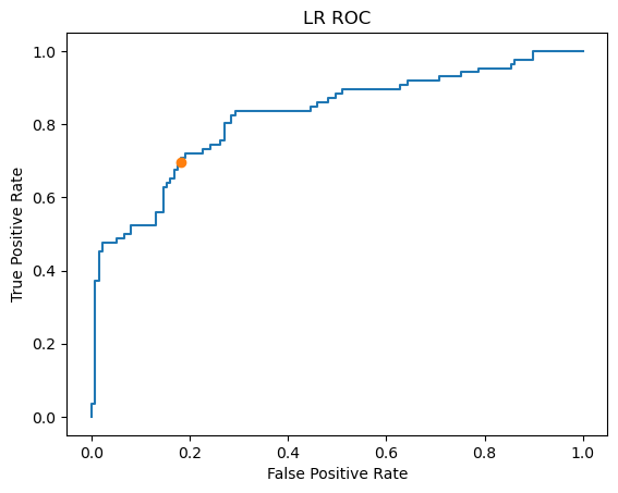
# ROC曲线,全称为接收者操作特性曲线
# ROC曲线图像的横轴代表假阳性率(假正率),纵轴代表真阳性率(真正率)。
# ROC曲线越靠近左上角,分类模型的性能越好。ROC曲线的形状和位置可以反映分类器的性能。
# 通过比较ROC曲线下方的面积,可以确定模型的准确性
from sklearn.metrics import roc_curve#导入ROC画图模块
fpr,tpr,thresholds=roc_curve(y_test,lr.decision_function(X_test))
fpr,tpr,thresholds#用于判断正负类的边界值,猜中的比例越大越好,猜错的比例越小越好(即找最靠近0的数的值预测效果最好)
(array([0.        , 0.        , 0.        , 0.00729927, 0.00729927,
        0.01459854, 0.01459854, 0.02189781, 0.02189781, 0.05109489,
        0.05109489, 0.06569343, 0.06569343, 0.08029197, 0.08029197,
        0.13138686, 0.13138686, 0.1459854 , 0.1459854 , 0.15328467,
        0.15328467, 0.16058394, 0.16058394, 0.16788321, 0.16788321,
        0.17518248, 0.17518248, 0.18248175, 0.18248175, 0.18978102,
        0.18978102, 0.22627737, 0.22627737, 0.24087591, 0.24087591,
        0.26277372, 0.26277372, 0.27007299, 0.27007299, 0.28467153,
        0.28467153, 0.2919708 , 0.2919708 , 0.44525547, 0.44525547,
        0.45985401, 0.45985401, 0.48175182, 0.48175182, 0.49635036,
        0.49635036, 0.51094891, 0.51094891, 0.62773723, 0.62773723,
        0.64233577, 0.64233577, 0.7080292 , 0.7080292 , 0.75182482,
        0.75182482, 0.78832117, 0.78832117, 0.8540146 , 0.8540146 ,
        0.86131387, 0.86131387, 0.89781022, 0.89781022, 1.        ]),
 array([0.        , 0.01162791, 0.03488372, 0.03488372, 0.37209302,
        0.37209302, 0.45348837, 0.45348837, 0.47674419, 0.47674419,
        0.48837209, 0.48837209, 0.5       , 0.5       , 0.52325581,
        0.52325581, 0.55813953, 0.55813953, 0.62790698, 0.62790698,
        0.63953488, 0.63953488, 0.65116279, 0.65116279, 0.6744186 ,
        0.6744186 , 0.69767442, 0.69767442, 0.70930233, 0.70930233,
        0.72093023, 0.72093023, 0.73255814, 0.73255814, 0.74418605,
        0.74418605, 0.75581395, 0.75581395, 0.80232558, 0.80232558,
        0.8255814 , 0.8255814 , 0.8372093 , 0.8372093 , 0.84883721,
        0.84883721, 0.86046512, 0.86046512, 0.87209302, 0.87209302,
        0.88372093, 0.88372093, 0.89534884, 0.89534884, 0.90697674,
        0.90697674, 0.91860465, 0.91860465, 0.93023256, 0.93023256,
        0.94186047, 0.94186047, 0.95348837, 0.95348837, 0.96511628,
        0.96511628, 0.97674419, 0.97674419, 1.        , 1.        ]),
 array([ 4.4604173 ,  3.4604173 ,  3.27475467,  3.13564037,  1.24456838,
         1.23741707,  1.04201006,  0.97150355,  0.86036255,  0.76794951,
         0.74231523,  0.65578192,  0.61321112,  0.59089726,  0.57737495,
         0.50079627,  0.48350023,  0.46786188,  0.4055465 ,  0.39454437,
         0.37323985,  0.35766549,  0.31694781,  0.31295873,  0.27574868,
         0.24584607,  0.14447573,  0.01849733, -0.15356221, -0.33429778,
        -0.35241676, -0.44643233, -0.46562561, -0.48065651, -0.60202748,
        -0.63136615, -0.63441685, -0.69163594, -0.77086181, -0.80384297,
        -0.91523124, -0.94550624, -0.95078796, -1.50292374, -1.57149891,
        -1.65211024, -1.66598834, -1.74991745, -1.76999817, -1.79121369,
        -1.79584672, -1.83853105, -1.84052955, -1.95917003, -1.97591619,
        -1.98861251, -1.99154742, -2.06071338, -2.06752118, -2.10658164,
        -2.11240595, -2.16204106, -2.16423123, -2.22073334, -2.22203828,
        -2.2400868 , -2.25233915, -2.29905826, -2.30682056, -2.96452693]))
plt.plot(fpr,tpr)#横坐标fpr,纵坐标tpr
plt.xlabel('False Positive Rate')
plt.ylabel('True Positive Rate')
Text(0, 0.5, 'True Positive Rate')
a=np.abs(thresholds)#绝对值
a
array([4.4604173 , 3.4604173 , 3.27475467, 3.13564037, 1.24456838,
       1.23741707, 1.04201006, 0.97150355, 0.86036255, 0.76794951,
       0.74231523, 0.65578192, 0.61321112, 0.59089726, 0.57737495,
       0.50079627, 0.48350023, 0.46786188, 0.4055465 , 0.39454437,
       0.37323985, 0.35766549, 0.31694781, 0.31295873, 0.27574868,
       0.24584607, 0.14447573, 0.01849733, 0.15356221, 0.33429778,
       0.35241676, 0.44643233, 0.46562561, 0.48065651, 0.60202748,
       0.63136615, 0.63441685, 0.69163594, 0.77086181, 0.80384297,
       0.91523124, 0.94550624, 0.95078796, 1.50292374, 1.57149891,
       1.65211024, 1.66598834, 1.74991745, 1.76999817, 1.79121369,
       1.79584672, 1.83853105, 1.84052955, 1.95917003, 1.97591619,
       1.98861251, 1.99154742, 2.06071338, 2.06752118, 2.10658164,
       2.11240595, 2.16204106, 2.16423123, 2.22073334, 2.22203828,
       2.2400868 , 2.25233915, 2.29905826, 2.30682056, 2.96452693])
close_zero=np.argmin(a)#找到最靠近0的数
close_zero#找出的数为预测效果最好的位置
27
plt.plot(fpr,tpr)#横坐标fpr,纵坐标tpr
plt.xlabel('False Positive Rate')
plt.ylabel('True Positive Rate')
plt.plot(fpr[close_zero],tpr[close_zero],'o')#标出预测效果最好的点
plt.title('LR ROC')
Text(0.5, 1.0, 'LR ROC')
from sklearn.metrics import plot_roc_curve#该模块可以直接画出ROC曲线
lr=LogisticRegression().fit(X_train,y_train)
lr1=LogisticRegression(C=1000).fit(X_train,y_train)
lr2=LogisticRegression(class_weight='balanced').fit(X_train,y_train)
lr_display=plot_roc_curve(lr,X_test,y_test,name='LR',response_method='decision_function')
plot_roc_curve(lr1,X_test,y_test,name='LR1',response_method='decision_function',ax=lr_display.ax_)
plot_roc_curve(lr2,X_test,y_test,name='LR2',response_method='decision_function',ax=lr_display.ax_)#将三个曲线叠加在一起(记得加.ax_)
C:\Users\17006\anaconda3\lib\site-packages\sklearn\linear_model\_logistic.py:444: ConvergenceWarning: lbfgs failed to converge (status=1):
STOP: TOTAL NO. of ITERATIONS REACHED LIMIT.

Increase the number of iterations (max_iter) or scale the data as shown in:
    https://scikit-learn.org/stable/modules/preprocessing.html
Please also refer to the documentation for alternative solver options:
    https://scikit-learn.org/stable/modules/linear_model.html#logistic-regression
  n_iter_i = _check_optimize_result(
C:\Users\17006\anaconda3\lib\site-packages\sklearn\utils\deprecation.py:87: FutureWarning: Function plot_roc_curve is deprecated; Function :func:`plot_roc_curve` is deprecated in 1.0 and will be removed in 1.2. Use one of the class methods: :meth:`sklearn.metrics.RocCurveDisplay.from_predictions` or :meth:`sklearn.metrics.RocCurveDisplay.from_estimator`.
  warnings.warn(msg, category=FutureWarning)


<sklearn.metrics._plot.roc_curve.RocCurveDisplay at 0x1fcacc0d750>
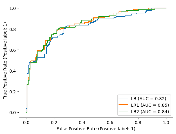
#AUC是曲线下的面积,面积越大效果越好(如图效果最好的是LR1)