第一章:sklearn总体介绍
引言
来自:https://www.heywhale.com/mw/project/63a306f9f000f7ef39f84e30
Sklearn (全称 Scikit-Learn) 是基于 Python 语言的机器学习工具。它建立在 NumPy, SciPy, Pandas 和 Matplotlib 之上,里面的 API 的设计非常好,所有对象的接口简单,很适合新手上路。
在 Sklearn 里面有六大任务模块:分别是分类、回归、聚类、降维、模型选择和预处理,如下图从其官网的截屏。

要使用上述六大模块的方法,可以用以下的伪代码,注意 import 后面我用的都是一些通用名称,如 SomeClassifier, SomeRegressor, SomeModel,具体化的名称由具体问题而定,比如
-
SomeClassifier = RandomForestClassifier
-
SomeRegressor = LinearRegression
-
SomeModel = KMeans, PCA
-
SomeModel = GridSearchCV, OneHotEncoder
上面具体化的例子分别是随机森林分类器、线性回归器、K 均值聚类、主成分分析、网格追踪法、独热编码。
-
分类 (Classification)
from sklearn import SomeClassifier
from sklearn.linear_model import SomeClassifier
from sklearn.ensemble import SomeClassifier -
回归 (Regression)
from sklearn import SomeRegressor
from sklearn.linear_model import SomeRegressor
from sklearn.ensemble import SomeRegressor -
聚类 (Clustering)
from sklearn.cluster import SomeModel -
降维 (Dimensionality Reduction)
from sklearn.decomposition import SomeModel -
模型选择 (Model Selection)
from sklearn.model_selection import SomeModel -
预处理 (Preprocessing)
from sklearn.preprocessing import SomeModel
SomeClassifier, SomeRegressor, SomeModel 其实都叫做估计器 (estimator),就像 Python 里「万物皆对象」那样,Sklearn 里「万物皆估计器」。
此外,Sklearn 里面还有很多自带数据集供,引入它们的伪代码如下。
数据集 (Dataset)
from sklearn.datasets import SomeData
本贴我们用以下思路来讲解:
第一章介绍机器学习,从定义出发引出机器学习四要素:数据、任务、性能度量和模型。加这一章的原因是不把机器学习相关概念弄清楚之后很难完全弄明白 Sklearn。
第二章介绍 Sklearn,从其 API 设计原理出发分析其五大特点:一致性、可检验、标准类、可组合和默认值。最后再分析 Sklearn 里面自带数据以及储存格式。
第三章介绍 Sklearn 里面的三大核心 API,包括估计器、预测器和转换器。这一章的内容最重要,几乎所有模型都会用到这三大 API。
第四章介绍 Sklearn 里面的高级 API,即元估计器,有可以大大简化代码量的流水线 (Pipeline 估计器),有集成模型 (Ensemble 估计器)、有多类别-多标签-多输出分类模型 (Multiclass 和 Multioutput 估计器) 和模型选择工具 (Model Selection 估计器)。
1 机器学习简介
1.1 定义和组成元素
什么是机器学习?字面上来讲就是 (人用) 计算机来学习。谈起机器学习就一定要提起汤姆米切尔 (Tom M.Mitchell),就像谈起音乐就会提起贝多芬,谈起篮球就会提起迈克尔乔丹,谈起电影就会提起莱昂纳多迪卡普里奥。米切尔对机器学习定义的原话是:
A computer program is said to learn from experience E with respect to some class of tasks T and performance measure P if its performance at tasks in T, as measured by P, improves with experience E.
整段英文有点抽象难懂对吗?首先注意到两个词 computer program 和 learn,翻译成中文就是机器 (计算机程序) 和学习,再把上面英译中:
假设用性能度量 P 来评估机器在某类任务 T 的性能,若该机器通利用经验 E 在任务 T 中改善其性能 P,那么可以说机器对经验 E 进行了学习。
在该定义中,除了核心词机器和学习,还有关键词经验 E,性能度量 P 和任务 T。在计算机系统中,通常经验 E 是以数据 D 的形式存在,而机器学习就是给定不同的任务 T 从数据中产生模型 M,模型 M 的好坏就用性能度量 P 来评估。
由上述机器学习的定义可知机器学习包含四个元素
数据 (Data)
任务 (Task)
性能度量 (Quality Metric)
模型 (Model)

下面四小节分别介绍数据、任务、性能度量和模型。
1.2 数据
数据 (data) 是经验的另一种说法,也是信息的载体。数据可分为
结构化数据和非结构化数据 (按数据具体类型划分)
原始数据和加工数据 (按数据表达形式划分)
样本内数据和样本外数据 (按数据统计性质划分)
结构化和非结构化
结构化数据 (structured data) 是由二维表结构来逻辑表达和实现的数据。非结构化数据是没有预定义的数据,不便用数据库二维表来表现的数据。
非结构化数据
非结构化数据包括图片,文字,语音和视屏等如下图。

对于以上的非结构数据,相关应用实例有
深度学习的卷积神经网络 (convolutional neural network, CNN) 对图像数据做人脸识别或物体分类
深度学习的循环神经网络 (recurrent neural network, RNN) 对语音数据做语音识别或机器对话,对文字数据做文本生成或阅读理解
增强学习的阿尔法狗 (AlphaGo) 对棋谱数据学习无数遍最终打败了围棋世界冠军李世石和柯洁
计算机追根到底还是只能最有效率的处理数值型的结构化数据,如何从原始数据加工成计算机可应用的数据会在后面讲明。
结构化数据
机器学习模型主要使用的是结构化数据,即二维的数据表。非结构化数据可以转换成结构化数据,比如把
图像类数据里像素张量重塑成一维数组
文本类数据用独热编码转成二维数组
对于结构化数据,我们用勒布朗詹姆斯 (Lebron James) 四场比赛的数据举例。

下面术语大家在深入了解机器学习前一定要弄清楚:
每行的记录 (这是一场比赛詹姆斯的个人统计) ,称为一个示例 (instance)
反映对象在某方面的性质,例如得分,篮板,助攻,称为特征 (feature) 或输入(input)
特征上的取值,例如「示例 1」对应的 27, 10, 12 称为特征值 (feature value)
关于示例结果的信息,例如赢,称为标签 (label) 或输出 (output)
包含标签信息的示例,则称为样例 (example),即样例 = (特征, 标签)
从数据中学得模型的过程称为学习 (learning) 或训练 (training)
在训练数据中,每个样例称为训练样例 (training example),整个集合称为训练集(training set)
1.3 任务
根据学习的任务模式 (训练数据是否有标签),机器学习可分为四大类:
有监督学习 (有标签)
无监督学习 (无标签)
半监督学习 (有部分标签)
增强学习 (有评级标签)
深度学习只是一种方法,而不是任务模式,因此与上面四类不属于同一个维度,但是深度学习与它们可以叠加成:深度有监督学习、深度非监督学习、深度半监督学习和深度增强学习。迁移学习也是一种方法,也可以分类为有监督迁移学习、非监督迁移学习、半监督迁移学习和增强迁移学习。
下图画出机器学习各类之间的关系。

1.4 性能度量
回归和分类任务中最常见的误差函数以及一些有用的性能度量如下。

2. Sklearn 数据
Sklearn 和之前讨论的 NumPy, SciPy, Pandas, Matplotlib 相似,就是一个处理特殊任务的包,Sklearn 就是处理机器学习 (有监督学习和无监督学习) 的包,更精确的说,它里面有六个任务模块和一个数据引入模块:
有监督学习的分类任务
有监督学习的回归任务
无监督学习的聚类任务
无监督学习的降维任务
数据预处理任务
模型选择任务
数据引入
本节就来看看 Sklearn 里数据格式和自带数据集。
2.1 数据格式
在 Sklean 里,模型能即用的数据有两种形式:
Numpy 二维数组 (ndarray) 的稠密数据 (dense data),通常都是这种格式。
SciPy 矩阵 (scipy.sparse.matrix) 的稀疏数据 (sparse data),比如文本分析每个单词 (字典有 100000 个词) 做独热编码得到矩阵有很多 0,这时用 ndarray 就不合适了,太耗内存。
numpy中matrix类型数据:https://www.runoob.com/numpy/numpy-matrix.html
import numpy as np

a = np.arange(12).reshape(3,4)
import numpy.matlib
c = np.matlib.empty((2,2))
type(c)
numpy.matrix
2.2 自带数据集
Sklearn 里面有很多自带数据集供用户使用。
特例描述:
数据集包括 150 条鸢尾花的四个特征 (萼片长/宽和花瓣长/宽) 和三个类别。在盘 Seaborn 时是从 csv 文件读取的,本帖从 Sklearn 里面的 datasets 模块中引入,代码如下:
from sklearn.datasets import load_iris
iris = load_iris()

#数据是以「字典」格式存储的,看看 iris 的键有哪些。
iris.keys()
dict_keys(['data', 'target', 'target_names', 'DESCR', 'feature_names', 'filename'])
#具体感受一下 iris 数据中特征的大小、名称和前五个示例。
n_samples, n_features = iris.data.shape
print((n_samples, n_features))
print(iris.feature_names)
iris.data[0:5]
(150, 4)
['sepal length (cm)', 'sepal width (cm)', 'petal length (cm)', 'petal width (cm)']


array([[5.1, 3.5, 1.4, 0.2],
       [4.9, 3. , 1.4, 0.2],
       [4.7, 3.2, 1.3, 0.2],
       [4.6, 3.1, 1.5, 0.2],
       [5. , 3.6, 1.4, 0.2]])
#150 个样本,4 个特征,没毛病!再感受一下标签的大小、名称和全部示例。
print(iris.target.shape)
print(iris.target_names)
iris.target
(150,)
['setosa' 'versicolor' 'virginica']


array([0, 0, 0, 0, 0, 0, 0, 0, 0, 0, 0, 0, 0, 0, 0, 0, 0, 0, 0, 0, 0, 0,
       0, 0, 0, 0, 0, 0, 0, 0, 0, 0, 0, 0, 0, 0, 0, 0, 0, 0, 0, 0, 0, 0,
       0, 0, 0, 0, 0, 0, 1, 1, 1, 1, 1, 1, 1, 1, 1, 1, 1, 1, 1, 1, 1, 1,
       1, 1, 1, 1, 1, 1, 1, 1, 1, 1, 1, 1, 1, 1, 1, 1, 1, 1, 1, 1, 1, 1,
       1, 1, 1, 1, 1, 1, 1, 1, 1, 1, 1, 1, 2, 2, 2, 2, 2, 2, 2, 2, 2, 2,
       2, 2, 2, 2, 2, 2, 2, 2, 2, 2, 2, 2, 2, 2, 2, 2, 2, 2, 2, 2, 2, 2,
       2, 2, 2, 2, 2, 2, 2, 2, 2, 2, 2, 2, 2, 2, 2, 2, 2, 2])
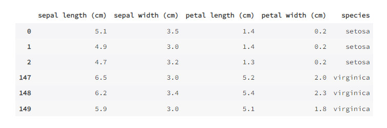
#用 Pandas 的 DataFrame (将 X 和 y 合并) 和 Seaborn 的 pairplot (看每个特征之间的关系) 来用表格和图来展示一下数据集的内容。
import pandas as pd
import seaborn as sns
iris_data = pd.DataFrame( iris.data,
                          columns=iris.feature_names )
iris_data['species'] = iris.target_names[iris.target]
iris_data.head(3).append(iris_data.tail(3))
Matplotlib is building the font cache using fc-list. This may take a moment.
sns.pairplot( iris_data, hue='species', palette='husl' );

正规引入
看完鸢尾花的 iris 数据展示后,现在来看看 Sklearn 三种引入数据形式。
打包好的数据:对于小数据集,用 sklearn.datasets.load_*
分流下载数据:对于大数据集,用 sklearn.datasets.fetch_*
随机创建数据:为了快速展示,用 sklearn.datasets.make_*
上面这个星号 * 是什么意思,指的是具体文件名,敲完
datasets.load_
datasets.fetch_
datasets.make_
from sklearn import datasets
datasets.load_iris
<function sklearn.datasets.base.load_iris(return_X_y=False)>
#Load 一个数字小数据集 digits?
digits = datasets.load_digits()
digits.keys()
dict_keys(['data', 'target', 'target_names', 'images', 'DESCR'])
#Fetch 一个加州房屋大数据集 california_housing?
california_housing = datasets.fetch_california_housing()
california_housing.keys()
Downloading Cal. housing from https://ndownloader.figshare.com/files/5976036 to /home/kesci/scikit_learn_data


dict_keys(['data', 'target', 'feature_names', 'DESCR'])
3. 核心 API
Sklearn 里万物皆估计器。估计器是个非常抽象的叫法,可把它不严谨的当成一个模型 (用来回归、分类、聚类、降维),或当成一套流程 (预处理、网格最终)。
本节三大 API 其实都是估计器:
估计器 (estimator) 当然是估计器
预测器 (predictor) 是具有预测功能的估计器
转换器 (transformer) 是具有转换功能的估计器
这三句看似废话,其实蕴藏了很多内容。其实我对第 1 点这个估计器的起名不太满意,我觉得应该叫拟合器 (fitter) - 具有拟合功能的估计器。看完这一节你就会明白「拟合器」这种叫法更合理。
3.1 估计器
定义:任何可以基于数据集对一些参数进行估计的对象都被称为估计器。
两个核心点:1. 需要输入数据,2. 可以估计参数。估计器首先被创建,然后被拟合。
创建估计器:需要设置一组超参数,比如
线性回归里超参数 normalize=True
K 均值里超参数 n_clusters=3
在创建好的估计器 model 可以直接访问这些超参数,用 . 符号。
model.normalize
model.n_clusters
但 model 中有很多超参数,你不可能一开始都知道要设置什么值,没设置的用 Sklearn 会给个合理的默认值,因此新手不用担心。
拟合估计器:需要训练集。在有监督学习中的代码范式为
model.fit( X_train, y_train )
在无监督学习中的代码范式为
model.fit( X_train )
拟合之后可以访问 model 里学到的参数,比如线性回归里的特征前的系数 coef_,或 K 均值里聚类标签 labels_。
model.coef_
model.labels_
说了这么多抽象的东西,现在展示有监督学习的「线性回归」和无监督学习的「K 均值」的具体例子。
线性回归
首先从 sklearn 下的 linear_model 中引入 LinearRegression,再创建估计器起名 model,设置超参数 normalize 为 True,指的在每个特征值上做标准化,这样会加速数值运算。
from sklearn.linear_model import LinearRegression
model = LinearRegression(normalize=True)
model
LinearRegression(copy_X=True, fit_intercept=True, n_jobs=None, normalize=True)
创建完后的估计器会显示所有的超参数,比如我们设置好的 normalize=True,其他没设置的都是去默认值,比如 n_jobs=None 是只用一个核,你可以将其设为 2 就是两核并行,甚至设为 -1 就是电脑里所有核并行。
自己创建一个简单数据集 (没有噪声完全线性) 只为了讲解估计器里面的特征。
import numpy as np
import matplotlib.pyplot as plt
x = np.arange(10)
y = 2 * x + 1
plt.plot( x, y, 'o' );

还记得 Sklearn 里模型要求特征 X 是个两维变量么 (样本数×特征数)?但在本例中 X 是一维,因为我们用 np.newaxis 加一个维度,它做的事情就是把 [1, 2, 3] 转成 [[1],[2],[3]]。再把 X 和 y 丢进 fit() 函数来拟合线性模型的参数。
X = x[:, np.newaxis]
model.fit( X, y )
LinearRegression(copy_X=True, fit_intercept=True, n_jobs=None, normalize=True)
拟合完后的估计器和创建完的样子看起来一样,但是已经用「model.param_」可以访问到学好的参数了,展示如下。
print( model.coef_ )
print( model.intercept_ )
[2.]
0.9999999999999982
K 均值
首先从 sklearn 下的 cluster 中引入 KMeans,再创建估计器起名 model,设置超参数 n_cluster 为 3 (为了展示方便而我们知道用的 iris 数据集有 3 类,实际上应该选不同数量的 n_cluster,根据 elbow 图来决定,下帖细讲)。
再者,iris 数据里是有标签 y 的,我们假装没有 y 才能无监督的聚类啊,要不然应该做有监督的分类的。
from sklearn.cluster import KMeans
model = KMeans( n_clusters=3 )
model
KMeans(algorithm='auto', copy_x=True, init='k-means++', max_iter=300,
       n_clusters=3, n_init=10, n_jobs=None, precompute_distances='auto',
       random_state=None, tol=0.0001, verbose=0)
创建完后的估计器会显示所有的超参数,比如我们设置好的 n_cluster=3,其他没设置的都是去默认值,比如 max_iter=300 是最多迭代次数为 300,算法不收敛也停了。
还记得 iris 里的特征有四个吗 (萼片长、萼片宽、花瓣长、花瓣宽)?四维特征很难可视化,因此我们只取两个特征 (萼片长、萼片宽) 来做聚类并且可视化结果。注意下面代码 X = iris.data[:,0:2]。
from sklearn.datasets import load_iris
iris = load_iris()
X = iris.data[:,0:2]
model.fit(X)
KMeans(algorithm='auto', copy_x=True, init='k-means++', max_iter=300,
       n_clusters=3, n_init=10, n_jobs=None, precompute_distances='auto',
       random_state=None, tol=0.0001, verbose=0)
拟合完后的估计器和创建完的样子看起来一样,但是已经用「model.param_」可以访问到学好的参数了,展示如下。
print( model.cluster_centers_, '\n')
print( model.labels_, '\n' )
print( model.inertia_, '\n')
print(iris.target)
[[5.77358491 2.69245283]
 [6.81276596 3.07446809]
 [5.006      3.428     ]]

[2 2 2 2 2 2 2 2 2 2 2 2 2 2 2 2 2 2 2 2 2 2 2 2 2 2 2 2 2 2 2 2 2 2 2 2 2
 2 2 2 2 2 2 2 2 2 2 2 2 2 1 1 1 0 1 0 1 0 1 0 0 0 0 0 0 1 0 0 0 0 0 0 0 0
 1 1 1 1 0 0 0 0 0 0 0 0 1 0 0 0 0 0 0 0 0 0 0 0 0 0 1 0 1 1 1 1 0 1 1 1 1
 1 1 0 0 1 1 1 1 0 1 0 1 0 1 1 0 0 1 1 1 1 1 0 0 1 1 1 0 1 1 1 0 1 1 1 0 1
 1 0]

37.05070212765958

[0 0 0 0 0 0 0 0 0 0 0 0 0 0 0 0 0 0 0 0 0 0 0 0 0 0 0 0 0 0 0 0 0 0 0 0 0
 0 0 0 0 0 0 0 0 0 0 0 0 0 1 1 1 1 1 1 1 1 1 1 1 1 1 1 1 1 1 1 1 1 1 1 1 1
 1 1 1 1 1 1 1 1 1 1 1 1 1 1 1 1 1 1 1 1 1 1 1 1 1 1 2 2 2 2 2 2 2 2 2 2 2
 2 2 2 2 2 2 2 2 2 2 2 2 2 2 2 2 2 2 2 2 2 2 2 2 2 2 2 2 2 2 2 2 2 2 2 2 2
 2 2]
有点乱,解释一下 KMeans 模型这几个参数:
model.cluster_centers_:簇中心。三个簇那么有三个坐标。
model.labels_:聚类后的标签
model.inertia_:所有点到对应的簇中心的距离平方和 (越小越好)
小结
虽然上面以有监督学习的 LinearRegression 和无监督学习的 KMeans 举例,但实际上你可以将它们替换成其他别的模型,比如有监督学习的 LogisticRegression 和无监督学习的 DBSCAN。它们都是「估计器」,因此都有 fit() 方法。使用它们的通用伪代码如下:
有监督学习
from sklearn.xxx import SomeModel
xxx 可以是 linear_model 或 ensemble 等
model = SomeModel( hyperparameter )
model.fit( X, y )
无监督学习
from sklearn.xxx import SomeModel
xxx 可以是 cluster 或 decomposition 等
model = SomeModel( hyperparameter )
model.fit( X )
3.2 预测器
定义:预测器在估计器上做了一个延展,延展出预测的功能。
两个核心点:1. 基于学到的参数预测,2. 预测有很多指标。最常见的就是 predict() 函数:
model.predict(X_test):评估模型在新数据上的表现
model.predict(X_train):确认模型在老数据上的表现
因为要做预测,首先将数据分成 80:20 的训练集 (X_train, y_train) 和测试集 (X_test, y_test),在用从训练集上拟合 fit() 的模型在测试集上预测 predict()。
from sklearn.datasets import load_iris
iris = load_iris()
from sklearn.model_selection import train_test_split
X_train, X_test, y_train, y_test = train_test_split( iris['data'],
                    iris['target'],
                    test_size=0.2 )
print( 'The size of X_train is ', X_train.shape )
print( 'The size of y_train is ', y_train.shape )
print( 'The size of X_test is ', X_test.shape )
print( 'The size of y_test is ', y_test.shape )
The size of X_train is  (120, 4)
The size of y_train is  (120,)
The size of X_test is  (30, 4)
The size of y_test is  (30,)
predict & predict_proba
对于分类问题,我们不仅想知道预测的类别是什么,有时还想知道预测该类别的信心如何。前者用 predict(),后者用 predict_proba()。
y_pred = model.predict( X_test )
p_pred = model.predict_proba( X_test )
print( y_test, '\n' )
print( y_pred, '\n' )
print( p_pred )
score & decision_function
预测器里还有额外的两个函数可以使用。在分类问题中
score() 返回的是分类准确率
decision_function() 返回的是每个样例在每个类下的分数值
print( model.score( X_test, y_test ) )
print( np.sum(y_pred==y_test)/len(y_test) )
decision_score = model.decision_function( X_test )
print( decision_score )
小节
估计器都有 fit() 方法,预测器都有 predict() 和 score() 方法,言外之意不是每个预测器都有 predict_proba() 和 decision_function() 方法,这个在用的时候查查官方文档就清楚了 (比如 RandomForestClassifier 就没有 decision_function() 方法)。
使用它们的通用伪代码如下:
有监督学习
from sklearn.xxx import SomeModel
xxx 可以是 linear_model 或 ensemble 等
model = SomeModel( hyperparameter )
model.fit( X, y )
y_pred = model.predict( X_new )
s = model.score( X_new )
无监督学习
from sklearn.xxx import SomeModel
xxx 可以是 cluster 或 decomposition 等
model = SomeModel( hyperparameter )
model.fit( X )
idx_pred = model.predict( X_new )
s = model.score( X_new )
3.3 转换器
定义:转换器也是一种估计器,两者都带拟合功能,但估计器做完拟合来预测,而转换器做完拟合来转换。
核心点:估计器里 fit + predict,转换器里 fit + transform。
本节介绍两大类转换器
将分类型变量 (categorical) 编码成数值型变量 (numerical)
规范化 (normalize) 或标准化 (standardize) 数值型变量
分类型变量编码
LabelEncoder & OrdinalEncoder
LabelEncoder 和 OrdinalEncoder 都可以将字符转成数字,但是
LabelEncoder 的输入是一维,比如 1d ndarray
OrdinalEncoder 的输入是二维,比如 DataFrame
#首先给出要编码的列表 enc 和要解码的列表 dec。
enc = ['win','draw','lose','win']
dec = ['draw','draw','win']
#从 sklearn 下的 preprocessing 中引入 LabelEncoder,再创建转换器起名 LE,不需要设置任何超参数。
from sklearn.preprocessing import LabelEncoder
LE = LabelEncoder()
print(LE.fit(enc))
print( LE.classes_ )
print( LE.transform(dec) )
LabelEncoder()
['draw' 'lose' 'win']
[0 0 2]
除了LabelEncoder 能编码,OrdinalEncoder 也可以。首先从 sklearn 下的 preprocessing 中引入 OrdinalEncoder,再创建转换器起名 OE,不需要设置任何超参数。 下面结果和上面类似,就不再多解释了。
from sklearn.preprocessing import OrdinalEncoder
OE = OrdinalEncoder()
enc_DF = pd.DataFrame(enc)
dec_DF = pd.DataFrame(dec)
print( OE.fit(enc_DF) )
print( OE.categories_ )
print( OE.transform(dec_DF) )
OrdinalEncoder(categories='auto', dtype=<class 'numpy.float64'>)
[array(['draw', 'lose', 'win'], dtype=object)]
[[0.]
 [0.]
 [2.]]
上面这种编码的问题是,机器学习算法会认为两个临近的值比两个疏远的值要更相似。显然这样不对 (比如,0 和 1 比 0 和 2 距离更近,难道 draw 和 win 比 draw 和 lose更相似?)。
要解决这个问题,一个常见的方法是给每个分类创建一个二元属性,即独热编码 (one-hot encoding)。如何用它看下段。
OneHotEncoder
独热编码其实就是把一个整数用向量的形式表现。下图就是对数字 0-9 做独热编码。

转换器 OneHotEncoder 可以接受两种类型的输入:
用 LabelEncoder 编码好的一维数组
DataFrame
一. 用 LabelEncoder 编码好的一维数组 (元素为整数),重塑 (用 reshape(-1,1)) 成二维数组作为 OneHotEncoder 输入。
from sklearn.preprocessing import OneHotEncoder
OHE = OneHotEncoder()
num = LE.fit_transform( enc )
print( num )
OHE_y = OHE.fit_transform( num.reshape(-1,1) )
OHE_y
[2 0 1 2]


/opt/conda/lib/python3.6/site-packages/sklearn/preprocessing/_encoders.py:414: FutureWarning: The handling of integer data will change in version 0.22. Currently, the categories are determined based on the range [0, max(values)], while in the future they will be determined based on the unique values.
If you want the future behaviour and silence this warning, you can specify "categories='auto'".
In case you used a LabelEncoder before this OneHotEncoder to convert the categories to integers, then you can now use the OneHotEncoder directly.
  warnings.warn(msg, FutureWarning)


<4x3 sparse matrix of type '<class 'numpy.float64'>'
	with 4 stored elements in Compressed Sparse Row format>
上面结果解释如下
第 3 行打印出编码结果 [2 0 1 2]
第 5 行将其转成独热形式,输出是一个「稀疏矩阵」形式,因为实操中通常类别很多,因此就一步到位用稀疏矩阵来节省内存
想看该矩阵里具体内容,用 toarray() 函数。
OHE_y.toarray()
array([[0., 0., 1.],
       [1., 0., 0.],
       [0., 1., 0.],
       [0., 0., 1.]])
二. 用 DataFrame作为 OneHotEncoder 输入。
OHE = OneHotEncoder()
OHE.fit_transform( enc_DF ).toarray()
array([[0., 0., 1.],
       [1., 0., 0.],
       [0., 1., 0.],
       [0., 0., 1.]])
特征缩放
数据要做的最重要的转换之一是特征缩放 (feature scaling)。当输入的数值的量刚不同时,机器学习算法的性能都不会好。
具体来说,对于某个特征,我们有两种方法:
标准化 (standardization):每个维度的特征减去该特征均值,除以该维度的标准差。
规范化 (normalization):每个维度的特征减去该特征最小值,除以该特征的最大值与最小值之差。
MinMaxScaler
整套转换器「先创建再 fit 在 transform」的流程应该很清楚了。自己读下面代码看看是不是秒懂。唯一需要注意的就是输入 X 要求是两维。
from sklearn.preprocessing import MinMaxScaler
X = np.array( [0, 0.5, 1, 1.5, 2, 100] )
X_scale = MinMaxScaler().fit_transform( X.reshape(-1,1) )
X_scale
array([[0.   ],
       [0.005],
       [0.01 ],
       [0.015],
       [0.02 ],
       [1.   ]])
StandardScaler
牢记转换器「先创建再 fit 在 transform」的流程就行了。
from sklearn.preprocessing import StandardScaler
X_scale = StandardScaler().fit_transform( X.reshape(-1,1) )
X_scale
array([[-0.47424487],
       [-0.46069502],
       [-0.44714517],
       [-0.43359531],
       [-0.42004546],
       [ 2.23572584]])
警示: fit() 函数只能作用在训练集上,千万不要作用在测试集上,要不然你就犯了数据窥探的错误了!拿标准化举例,用训练集 fit 出来的均值和标准差参数,来对测试集做标准化。
4. 高级 API
Sklearn 里核心 API 接口是估计器,那高级 API 接口就是元估计器 (meta-estimator),即由很多基估计器 (base estimator) 组合成的估计器。
meta_model( base_model )
本节讨论五大元估计器,分别带集成功能的 ensemble,多分类和多标签的 multiclass,多输出的 multioutput,选择模型的 model_selection,和流水线的 pipeline。
ensemble.BaggingClassifier
ensemble.VotingClassifier
multiclass.OneVsOneClassifier
multiclass.OneVsRestClassifier
multioutput.MultiOutputClassifier
model_selection.GridSearchCV
model_selection.RandomizedSearchCV
pipeline.Pipeline
4.1 Ensemble 估计器
分类器统计每个子分类器的预测类别数,再用「多数投票」原则得到最终预测。
回归器计算每个子回归器的预测平均值。
最常用的 Ensemble 估计器排列如下:
AdaBoostClassifier: 逐步提升分类器
AdaBoostRegressor: 逐步提升回归器
BaggingClassifier: 装袋分类器
BaggingRegressor: 装袋回归器
GradientBoostingClassifier: 梯度提升分类器
GradientBoostingRegressor: 梯度提升回归器
RandomForestClassifier: 随机森林分类器
RandomForestRegressor: 随机森林回归器
VotingClassifier: 投票分类器
VotingRegressor: 投票回归器
我们用鸢尾花数据 iris,拿
含同质估计器 RandomForestClassifier
含异质估计器 VotingClassifier
来举例。首先将数据分成 80:20 的训练集和测试集,并引入 metrics 来计算各种性能指标。
from sklearn.datasets import load_iris
iris = load_iris()
from sklearn.model_selection import train_test_split
from sklearn import metrics
X_train, X_test, y_train, y_test = train_test_split(iris['data'], iris['target'], test_size=0.2)
RandomForestClassifier
RandomForestClassifier 通过控制 n_estimators 超参数来决定基估计器的个数,本例是 4 棵决策树 (森林由树组成);此外每棵树的最大树深为 5 (max_depth=5)。
from sklearn.ensemble import RandomForestClassifier
RF = RandomForestClassifier( n_estimators=4, max_depth=5 )
RF.fit( X_train, y_train )
RandomForestClassifier(bootstrap=True, class_weight=None, criterion='gini',
                       max_depth=5, max_features='auto', max_leaf_nodes=None,
                       min_impurity_decrease=0.0, min_impurity_split=None,
                       min_samples_leaf=1, min_samples_split=2,
                       min_weight_fraction_leaf=0.0, n_estimators=4,
                       n_jobs=None, oob_score=False, random_state=None,
                       verbose=0, warm_start=False)
估计器有 fit(),元估计器当然也有 fit()。在估计器那一套又可以照搬到元估计器 (起名 RF) 上了。看看 RF 里包含的估计器个数和其本身。
print( RF.n_estimators )
RF.estimators_
4


[DecisionTreeClassifier(class_weight=None, criterion='gini', max_depth=5,
                        max_features='auto', max_leaf_nodes=None,
                        min_impurity_decrease=0.0, min_impurity_split=None,
                        min_samples_leaf=1, min_samples_split=2,
                        min_weight_fraction_leaf=0.0, presort=False,
                        random_state=705712365, splitter='best'),
 DecisionTreeClassifier(class_weight=None, criterion='gini', max_depth=5,
                        max_features='auto', max_leaf_nodes=None,
                        min_impurity_decrease=0.0, min_impurity_split=None,
                        min_samples_leaf=1, min_samples_split=2,
                        min_weight_fraction_leaf=0.0, presort=False,
                        random_state=1026568399, splitter='best'),
 DecisionTreeClassifier(class_weight=None, criterion='gini', max_depth=5,
                        max_features='auto', max_leaf_nodes=None,
                        min_impurity_decrease=0.0, min_impurity_split=None,
                        min_samples_leaf=1, min_samples_split=2,
                        min_weight_fraction_leaf=0.0, presort=False,
                        random_state=1987322366, splitter='best'),
 DecisionTreeClassifier(class_weight=None, criterion='gini', max_depth=5,
                        max_features='auto', max_leaf_nodes=None,
                        min_impurity_decrease=0.0, min_impurity_split=None,
                        min_samples_leaf=1, min_samples_split=2,
                        min_weight_fraction_leaf=0.0, presort=False,
                        random_state=1210538094, splitter='best')]
拟合 RF 完再做预测,用 metrics 里面的 accuracy_score 来计算准确率。训练准确率 98.33%,测试准确率 100%。
print ( "RF - Accuracy (Train):  %.4g" %
        metrics.accuracy_score(y_train, RF.predict(X_train)) )
print ( "RF - Accuracy (Test):  %.4g" %
        metrics.accuracy_score(y_test, RF.predict(X_test)) )
RF - Accuracy (Train):  1
RF - Accuracy (Test):  0.9667
参考:https://blog.csdn.net/algorithmPro/article/details/103045824
第二章:sklearn实战练习
https://www.heywhale.com/mw/project/5df87b152823a10036aca1a9
参考:
中文手册:https://sklearn.apachecn.org/#/docs/master/2
在线练习:
https://www.heywhale.com/mw/project/63a306f9f000f7ef39f84e30
https://www.heywhale.com/mw/project/5df87b152823a10036aca1a9
第100章:skearn常见函数讲解:
sklearn.utils.shuffles使用:
https://blog.csdn.net/qq_41664939/article/details/123293310